

208
13 Cosmological Preliminaries
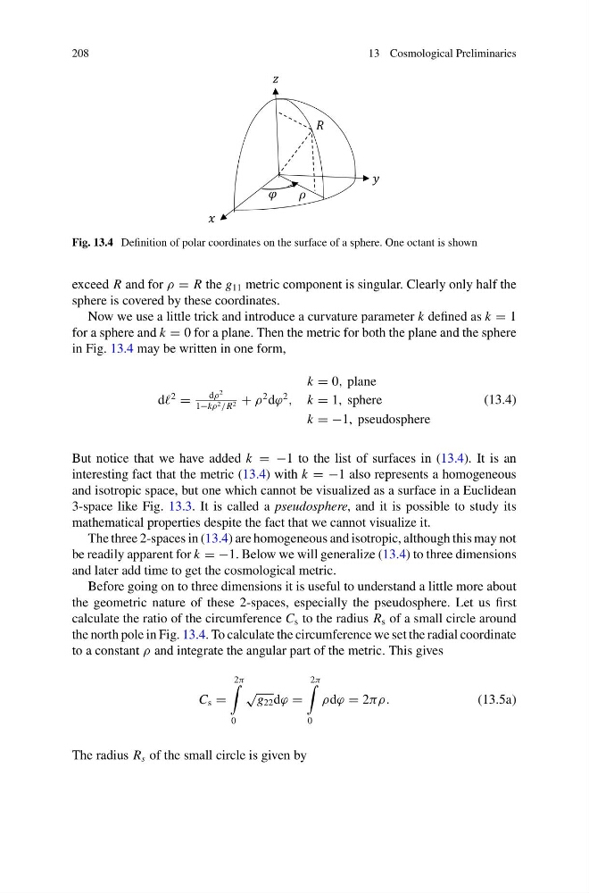
Fig. 13.4 Definition of polar coordinates on the surface of a sphere. One octant is shown
exceed R and for ρ = R the g 11 metric component is singular. Clearly only half the
sphere is covered by these coordinates.
Now we use a little trick and introduce a curvature parameter k defined as k = 1
for a sphere and k = 0 for a plane. Then the metric for both the plane and the sphere
in Fig. 13.4 may be written in one form,
k = 0, plane
d
2
=
dρ
2
1−kρ 2 /R 2 + ρ
2 dϕ
2
, k = 1, sphere
k = −1, pseudosphere
(13.4)
But notice that we have added k = −1 to the list of surfaces in (13.4). It is an
interesting fact that the metric (13.4) with k = −1 also represents a homogeneous
and isotropic space, but one which cannot be visualized as a surface in a Euclidean
3-space like Fig. 13.3. It is called a pseudosphere, and it is possible to study its
mathematical properties despite the fact that we cannot visualize it.
The three 2-spaces in (13.4) are homogeneous and isotropic, although this may not
be readily apparent for k = −1. Below we will generalize (13.4) to three dimensions
and later add time to get the cosmological metric.
Before going on to three dimensions it is useful to understand a little more about
the geometric nature of these 2-spaces, especially the pseudosphere. Let us first
calculate the ratio of the circumference C s to the radius R s of a small circle around
the north pole in Fig. 13.4. To calculate the circumference we set the radial coordinate
to a constant ρ and integrate the angular part of the metric. This gives
C s =
2π
0
√ g 22 dϕ =
2π
0
ρdϕ = 2πρ.
(13.5a)
The radius R s of the small circle is given by
13 Cosmological Preliminaries
Fig. 13.4 Definition of polar coordinates on the surface of a sphere. One octant is shown
exceed R and for ρ = R the g 11 metric component is singular. Clearly only half the
sphere is covered by these coordinates.
Now we use a little trick and introduce a curvature parameter k defined as k = 1
for a sphere and k = 0 for a plane. Then the metric for both the plane and the sphere
in Fig. 13.4 may be written in one form,
k = 0, plane
d
2
=
dρ
2
1−kρ 2 /R 2 + ρ
2 dϕ
2
, k = 1, sphere
k = −1, pseudosphere
(13.4)
But notice that we have added k = −1 to the list of surfaces in (13.4). It is an
interesting fact that the metric (13.4) with k = −1 also represents a homogeneous
and isotropic space, but one which cannot be visualized as a surface in a Euclidean
3-space like Fig. 13.3. It is called a pseudosphere, and it is possible to study its
mathematical properties despite the fact that we cannot visualize it.
The three 2-spaces in (13.4) are homogeneous and isotropic, although this may not
be readily apparent for k = −1. Below we will generalize (13.4) to three dimensions
and later add time to get the cosmological metric.
Before going on to three dimensions it is useful to understand a little more about
the geometric nature of these 2-spaces, especially the pseudosphere. Let us first
calculate the ratio of the circumference C s to the radius R s of a small circle around
the north pole in Fig. 13.4. To calculate the circumference we set the radial coordinate
to a constant ρ and integrate the angular part of the metric. This gives
C s =
2π
0
√ g 22 dϕ =
2π
0
ρdϕ = 2πρ.
(13.5a)
The radius R s of the small circle is given by