

184
11 Linearized General Relativity and Gravitational Waves
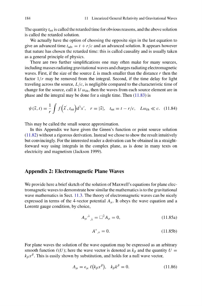
The quantity t ret is called the retarded time for obvious reasons, and the above solution
is called the retarded solution.
We actually have the option of choosing the opposite sign in the last equation to
give an advanced time t adv = t + r/c and an advanced solution. It appears however
that nature has chosen the retarded time: this is called causality and is usually taken
as a general principle of physics.
There are two further simplifications one may often make for many sources,
including masses radiating gravitational waves and charges radiating electromagnetic
waves. First, if the size of the source L is much smaller than the distance r then the
factor 1/r may be removed from the integral. Second, if the time delay for light
traveling across the source, L/c, is negligible compared to the characteristic time of
change for the source, call it 1/ ω ch , then the waves from each source element are in
phase and the integral may be done for a single time. Then (11.83) is
ψ( x, t) =
1
r
f
x
, t ret
d
3 x
, r = | x|, t ret = t − r/c, Lω ch c. (11.84)
This may be called the small source approximation.
In this Appendix we have given the Green’s function or point source solution
(11.82) without a rigorous derivation. Instead we chose to show the result intuitively
but convincingly. For the interested reader a derivation can be obtained in a straightforward way using integrals in the complex plane, as is done in many texts on
electricity and magnetism (Jackson 1999).
Appendix 2: Electromagnetic Plane Waves
We provide here a brief sketch of the solution of Maxwell’s equations for plane electromagnetic waves to demonstrate how similar the mathematics is to the gravitational
wave mathematics in Sect. 11.3. The theory of electromagnetic waves can be nicely
expressed in terms of the 4-vector potential A μ . It obeys the wave equation and a
Lorentz gauge condition, by choice,
A μ
,λ
,λ =
2 A μ = 0,
(11.85a)
A
ν ,ν = 0.
(11.85b)
For plane waves the solution of the wave equation may be expressed as an arbitrary
smooth function (U ); here the wave vector is denoted as k β and the quantity U =
k β x
β . This is easily shown by substitution, and holds for a null wave vector,
A μ = μ
k β x
β
, k β k
β
= 0.
(11.86)
11 Linearized General Relativity and Gravitational Waves
The quantity t ret is called the retarded time for obvious reasons, and the above solution
is called the retarded solution.
We actually have the option of choosing the opposite sign in the last equation to
give an advanced time t adv = t + r/c and an advanced solution. It appears however
that nature has chosen the retarded time: this is called causality and is usually taken
as a general principle of physics.
There are two further simplifications one may often make for many sources,
including masses radiating gravitational waves and charges radiating electromagnetic
waves. First, if the size of the source L is much smaller than the distance r then the
factor 1/r may be removed from the integral. Second, if the time delay for light
traveling across the source, L/c, is negligible compared to the characteristic time of
change for the source, call it 1/ ω ch , then the waves from each source element are in
phase and the integral may be done for a single time. Then (11.83) is
ψ( x, t) =
1
r
f
x
, t ret
d
3 x
, r = | x|, t ret = t − r/c, Lω ch c. (11.84)
This may be called the small source approximation.
In this Appendix we have given the Green’s function or point source solution
(11.82) without a rigorous derivation. Instead we chose to show the result intuitively
but convincingly. For the interested reader a derivation can be obtained in a straightforward way using integrals in the complex plane, as is done in many texts on
electricity and magnetism (Jackson 1999).
Appendix 2: Electromagnetic Plane Waves
We provide here a brief sketch of the solution of Maxwell’s equations for plane electromagnetic waves to demonstrate how similar the mathematics is to the gravitational
wave mathematics in Sect. 11.3. The theory of electromagnetic waves can be nicely
expressed in terms of the 4-vector potential A μ . It obeys the wave equation and a
Lorentz gauge condition, by choice,
A μ
,λ
,λ =
2 A μ = 0,
(11.85a)
A
ν ,ν = 0.
(11.85b)
For plane waves the solution of the wave equation may be expressed as an arbitrary
smooth function (U ); here the wave vector is denoted as k β and the quantity U =
k β x
β . This is easily shown by substitution, and holds for a null wave vector,
A μ = μ
k β x
β
, k β k
β
= 0.
(11.86)