

Appendix 1: Solutions for Retarded Potentials
183
2
ψ( x, t) = 4π f ( x, t),
2
≡ η
αβ ∂
∂ x α
∂
∂ x β =
∂
2
∂t 2 − ∇
2
.
(11.78)
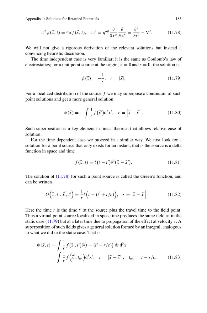
We will not give a rigorous derivation of the relevant solutions but instead a
convincing heuristic discussion.
The time independent case is very familiar; it is the same as Coulomb’s law of
electrostatics; for a unit point source at the origin,
x = 0 and r = 0, the solution is
ψ( x) = −
1
r
, r = | x|.
(11.79)
For a localized distribution of the source f we may superpose a continuum of such
point solutions and get a more general solution
ψ( x) = −
1
r
f
x
d
3 x
, r =
x − −
x
.
(11.80)
Such superposition is a key element in linear theories that allows relative ease of
solution.
For the time dependent case we proceed in a similar way. We first look for a
solution for a point source that only exists for an instant, that is the source is a delta
function in space and time
f ( x, t) = δ
t − t
δ
3
x − −
x
.
(11.81)
The solution of (11.78) for such a point source is called the Green’s function, and
can be written
G
x, t : :
x
, t
=
1
r
δ
t − (t
+ r/c)
, r =
x − −
x
.
(11.82)
Here the time t is the time t
at the source plus the travel time to the field point.
Thus a virtual point source localized in spacetime produces the same field as in the
static case (11.79) but at a later time due to propagation of the effect at velocity c. A
superposition of such fields gives a general solution formed by an integral, analogous
to what we did in the static case. That is
ψ( x, t) =
1
r
f
x
, t
δ
t − (t
+ r/c)
dt d
3 x
=
1
r
f
x
, t ret
d
3 x
, r =
x − −
x
, t ret = t − r/c.
(11.83)
183
2
ψ( x, t) = 4π f ( x, t),
2
≡ η
αβ ∂
∂ x α
∂
∂ x β =
∂
2
∂t 2 − ∇
2
.
(11.78)
We will not give a rigorous derivation of the relevant solutions but instead a
convincing heuristic discussion.
The time independent case is very familiar; it is the same as Coulomb’s law of
electrostatics; for a unit point source at the origin,
x = 0 and r = 0, the solution is
ψ( x) = −
1
r
, r = | x|.
(11.79)
For a localized distribution of the source f we may superpose a continuum of such
point solutions and get a more general solution
ψ( x) = −
1
r
f
x
d
3 x
, r =
x − −
x
.
(11.80)
Such superposition is a key element in linear theories that allows relative ease of
solution.
For the time dependent case we proceed in a similar way. We first look for a
solution for a point source that only exists for an instant, that is the source is a delta
function in space and time
f ( x, t) = δ
t − t
δ
3
x − −
x
.
(11.81)
The solution of (11.78) for such a point source is called the Green’s function, and
can be written
G
x, t : :
x
, t
=
1
r
δ
t − (t
+ r/c)
, r =
x − −
x
.
(11.82)
Here the time t is the time t
at the source plus the travel time to the field point.
Thus a virtual point source localized in spacetime produces the same field as in the
static case (11.79) but at a later time due to propagation of the effect at velocity c. A
superposition of such fields gives a general solution formed by an integral, analogous
to what we did in the static case. That is
ψ( x, t) =
1
r
f
x
, t
δ
t − (t
+ r/c)
dt d
3 x
=
1
r
f
x
, t ret
d
3 x
, r =
x − −
x
, t ret = t − r/c.
(11.83)