

176
11 Linearized General Relativity and Gravitational Waves
h 11 =
4G M
c 2 r
R
2
ω
2
c 2
cos 2ωt
1 + cos
2
θ
2
,
h 12 =
4G M
c 2 r
R
2
ω
2
c 2
sin 2ωt(cos θ ).
(11.67)
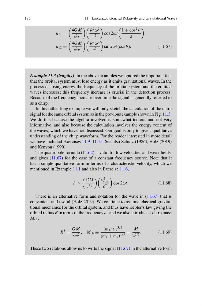
Example 11.3 (lengthy) In the above examples we ignored the important fact
that the orbital system must lose energy as it emits gravitational waves. In the
process of losing energy the frequency of the orbital system and the emitted
waves increases; this frequency increase is crucial in the detection process.
Because of the frequency increase over time the signal is generally referred to
as a chirp.
In this rather long example we will only sketch the calculation of the chirp
signal for the same orbital system as in the previous example shown in Fig. 11.3.
We do this because the algebra involved is somewhat tedious and not very
informative, and also because the calculation involves the energy content of
the waves, which we have not discussed. Our goal is only to give a qualitative
understanding of the chirp waveform. For the reader interested in more detail
we have included Exercises 11.9–11.15. See also Schutz (1986), Holz (2019)
and Kenyon (1990).
The quadrupole formula (11.62) is valid for low velocities and weak fields,
and gives (11.67) for the case of a constant frequency source. Note that it
has a simple qualitative form in terms of a characteristic velocity, which we
mentioned in Example 11.1 and also in Exercise 11.6,
h ∼
G M
c 2 r
v
2
char
c 2
cos 2ωt.
(11.68)
There is an alternative form and notation for the wave in (11.67) that is
convenient and useful (Holz 2019). We continue to assume classical gravitational mechanics for the orbital system, and thus have Kepler’s law giving the
orbital radius R in terms of the frequency ω, and we also introduce a chirp mass
M ch ,
R
3
=
G M
8ω 2 , M ch ≡
(m 1 m s )
3/5
(m 1 + m s )
1/5
=
M
2 6/5 ,
(11.69)
These two relations allow us to write the signal (11.67) in the alternative form
11 Linearized General Relativity and Gravitational Waves
h 11 =
4G M
c 2 r
R
2
ω
2
c 2
cos 2ωt
1 + cos
2
θ
2
,
h 12 =
4G M
c 2 r
R
2
ω
2
c 2
sin 2ωt(cos θ ).
(11.67)
Example 11.3 (lengthy) In the above examples we ignored the important fact
that the orbital system must lose energy as it emits gravitational waves. In the
process of losing energy the frequency of the orbital system and the emitted
waves increases; this frequency increase is crucial in the detection process.
Because of the frequency increase over time the signal is generally referred to
as a chirp.
In this rather long example we will only sketch the calculation of the chirp
signal for the same orbital system as in the previous example shown in Fig. 11.3.
We do this because the algebra involved is somewhat tedious and not very
informative, and also because the calculation involves the energy content of
the waves, which we have not discussed. Our goal is only to give a qualitative
understanding of the chirp waveform. For the reader interested in more detail
we have included Exercises 11.9–11.15. See also Schutz (1986), Holz (2019)
and Kenyon (1990).
The quadrupole formula (11.62) is valid for low velocities and weak fields,
and gives (11.67) for the case of a constant frequency source. Note that it
has a simple qualitative form in terms of a characteristic velocity, which we
mentioned in Example 11.1 and also in Exercise 11.6,
h ∼
G M
c 2 r
v
2
char
c 2
cos 2ωt.
(11.68)
There is an alternative form and notation for the wave in (11.67) that is
convenient and useful (Holz 2019). We continue to assume classical gravitational mechanics for the orbital system, and thus have Kepler’s law giving the
orbital radius R in terms of the frequency ω, and we also introduce a chirp mass
M ch ,
R
3
=
G M
8ω 2 , M ch ≡
(m 1 m s )
3/5
(m 1 + m s )
1/5
=
M
2 6/5 ,
(11.69)
These two relations allow us to write the signal (11.67) in the alternative form