

166
11 Linearized General Relativity and Gravitational Waves
ds
2
= c
2 dt
2
− (1 − h 11 )dx
2
− (1 + h 11 )dy
2
+ 2h 12 dxdy − dz
2
.
(11.29)
In the next section we will study the meaning of the two arbitrary functions in the
metric.
A comment on some basic physics is in order at this point: the metric obeys
the wave equation with velocity c so one might think that this shows the physical
gravitational field propagates at c. However, this is not the correct viewpoint since the
Riemann tensor is the intrinsic signature of gravity rather than the metric. But since
the Riemann tensor also obeys the wave equation with velocity c we can indeed
correctly say that the gravitational field propagates at c, at least in the weak field
approximation.
We have easily obtained the above as one convenient plane wave solution for the
metric field. It is important to also show that if one has any solution to the basic
(11.24) then it can be put into the form (11.28) by a gauge transformation, and most
important the gauge transformation can be obtained explicitly. This is very important
for the solutions we will obtain in the section below on sources of gravitational waves.
The remainder of this section will be devoted to showing in considerable algebraic
detail how to transform an arbitrary plane wave solution to the traceless transverse
form in (11.28) that serves as a canonical form.
The elements of the metric field as well as the gauge transformation functions
may all be taken to be functions of U = ct − z, as we have discussed above. The
Lorentz condition in (11.24) then strongly restricts the components of the metric,
giving
¯
h
μν
,ν = ¯
h
μ0
,0 + ¯
h
μ3
,3 = ¯
h
μ0
,U − ¯
h
μ3
,U =
¯
h
μ0
− ¯
h
μ3
,U
= 0.
(11.30)
Since the components ¯
h
μ0 and ¯
h
μ3 are functions of only the variable U they can
only differ by a constant; we will consider them equal since we are interested in time
varying wave fields rather than constant fields, and thus find
¯
h
μ0
= ¯
h
μ3
.
(11.31)
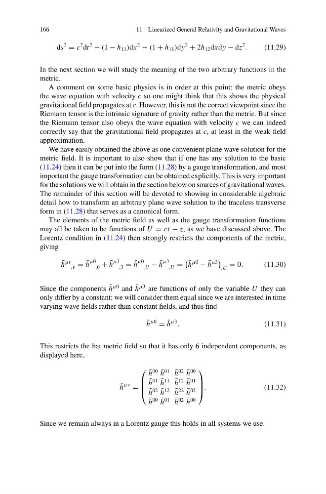
This restricts the hat metric field so that it has only 6 independent components, as
displayed here,
¯
h
μν
=
⎛
⎜
⎜
⎝
¯
h
00 ¯
h
01
¯
h
01 ¯
h
11
¯
h
02 ¯
h
00
¯
h
12 ¯
h
01
¯
h
02 ¯
h
12
¯
h
00 ¯
h
01
¯
h
22 ¯
h
02
¯
h
02 ¯
h
00
⎞
⎟
⎟
⎠ .
(11.32)
Since we remain always in a Lorentz gauge this holds in all systems we use.
11 Linearized General Relativity and Gravitational Waves
ds
2
= c
2 dt
2
− (1 − h 11 )dx
2
− (1 + h 11 )dy
2
+ 2h 12 dxdy − dz
2
.
(11.29)
In the next section we will study the meaning of the two arbitrary functions in the
metric.
A comment on some basic physics is in order at this point: the metric obeys
the wave equation with velocity c so one might think that this shows the physical
gravitational field propagates at c. However, this is not the correct viewpoint since the
Riemann tensor is the intrinsic signature of gravity rather than the metric. But since
the Riemann tensor also obeys the wave equation with velocity c we can indeed
correctly say that the gravitational field propagates at c, at least in the weak field
approximation.
We have easily obtained the above as one convenient plane wave solution for the
metric field. It is important to also show that if one has any solution to the basic
(11.24) then it can be put into the form (11.28) by a gauge transformation, and most
important the gauge transformation can be obtained explicitly. This is very important
for the solutions we will obtain in the section below on sources of gravitational waves.
The remainder of this section will be devoted to showing in considerable algebraic
detail how to transform an arbitrary plane wave solution to the traceless transverse
form in (11.28) that serves as a canonical form.
The elements of the metric field as well as the gauge transformation functions
may all be taken to be functions of U = ct − z, as we have discussed above. The
Lorentz condition in (11.24) then strongly restricts the components of the metric,
giving
¯
h
μν
,ν = ¯
h
μ0
,0 + ¯
h
μ3
,3 = ¯
h
μ0
,U − ¯
h
μ3
,U =
¯
h
μ0
− ¯
h
μ3
,U
= 0.
(11.30)
Since the components ¯
h
μ0 and ¯
h
μ3 are functions of only the variable U they can
only differ by a constant; we will consider them equal since we are interested in time
varying wave fields rather than constant fields, and thus find
¯
h
μ0
= ¯
h
μ3
.
(11.31)
This restricts the hat metric field so that it has only 6 independent components, as
displayed here,
¯
h
μν
=
⎛
⎜
⎜
⎝
¯
h
00 ¯
h
01
¯
h
01 ¯
h
11
¯
h
02 ¯
h
00
¯
h
12 ¯
h
01
¯
h
02 ¯
h
12
¯
h
00 ¯
h
01
¯
h
22 ¯
h
02
¯
h
02 ¯
h
00
⎞
⎟
⎟
⎠ .
(11.32)
Since we remain always in a Lorentz gauge this holds in all systems we use.