

8 Mössbauer Spectroscopy in External Magnetic Fields
389
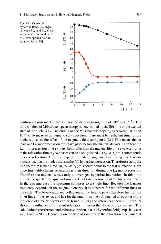
Fig. 8.7 Measured
hyperfine field B h f , angle
between B h f and B a , as well
as calculated internal field
B int over applied field B a .
Adapted from [19]
neutron measurements have a characteristic measuring time of 10
−8
− 10
−13 s. The
time window of Mössbauer spectroscopy is determined by the life time of the excited
state of the nucleus τ N . Depending on the Mössbauer isotope τ N is between 10
−7 and
10
−9 s. To measure a magnetic split spectrum, there must be sufficient time for the
nucleus to sense the effect of the magnetic field acting on it [21]. This means that at
least one Larmor precession must take place before the nucleus decays. Therefore the
Larmor precession time τ L must be smaller than the nucleus life time τ N . According
to the relaxation time τ R two cases can be distinguished. (i) τ R τ L ; this corresponds
to slow relaxation. Here the hyperfine fields change so slow during one Larmor
precession, that the nucleus senses the full hyperfine interaction. Therefore a static six
line spectrum is measured. (ii) τ R τ L ; this corresponds to the fast relaxation. Here
hyperfine fields change several times their direction during one Larmor precession.
Therefore the nucleus senses only an averaged hyperfine interaction. In this time
regime the spectra collapse and so-called motional narrowing of the lines take place.
In the extreme case the spectrum collapses to a single line. Because the Larmor
frequency depends on the magnetic energy, it is different for the different lines of
the sextet. The broadening and collapsing of the lines appears therefore first for the
inner lines of the sextet, and last for the outermost ones. A detailed discussion of the
influence of time windows can be found in [21] and references therein. Figure 8.9
shows the influence of different relaxation times on the shape of the spectrum. The
calculation is performed under the assumption that the hyperfine field jumps between
+20 T and −20 T. Depending on the type of sample and the relaxation mechanism it
389
Fig. 8.7 Measured
hyperfine field B h f , angle
between B h f and B a , as well
as calculated internal field
B int over applied field B a .
Adapted from [19]
neutron measurements have a characteristic measuring time of 10
−8
− 10
−13 s. The
time window of Mössbauer spectroscopy is determined by the life time of the excited
state of the nucleus τ N . Depending on the Mössbauer isotope τ N is between 10
−7 and
10
−9 s. To measure a magnetic split spectrum, there must be sufficient time for the
nucleus to sense the effect of the magnetic field acting on it [21]. This means that at
least one Larmor precession must take place before the nucleus decays. Therefore the
Larmor precession time τ L must be smaller than the nucleus life time τ N . According
to the relaxation time τ R two cases can be distinguished. (i) τ R τ L ; this corresponds
to slow relaxation. Here the hyperfine fields change so slow during one Larmor
precession, that the nucleus senses the full hyperfine interaction. Therefore a static six
line spectrum is measured. (ii) τ R τ L ; this corresponds to the fast relaxation. Here
hyperfine fields change several times their direction during one Larmor precession.
Therefore the nucleus senses only an averaged hyperfine interaction. In this time
regime the spectra collapse and so-called motional narrowing of the lines take place.
In the extreme case the spectrum collapses to a single line. Because the Larmor
frequency depends on the magnetic energy, it is different for the different lines of
the sextet. The broadening and collapsing of the lines appears therefore first for the
inner lines of the sextet, and last for the outermost ones. A detailed discussion of the
influence of time windows can be found in [21] and references therein. Figure 8.9
shows the influence of different relaxation times on the shape of the spectrum. The
calculation is performed under the assumption that the hyperfine field jumps between
+20 T and −20 T. Depending on the type of sample and the relaxation mechanism it