

3 Quantum Optical Phenomena in Nuclear Resonant Scattering
117
h ii = ω 0 −
i
2
and h i j (i = j) = −
γ
2
κ i j
e
ik 0 R i j
k 0 R i j
(3.12)
with
κ i j ≈
3
2
3 cos
2
− 1
1
(k 0 R i j ) 2 −
i
k 0 R i j
(near zone R i j λ)
3
2
sin
2
( far zone R i j λ)
(3.13)
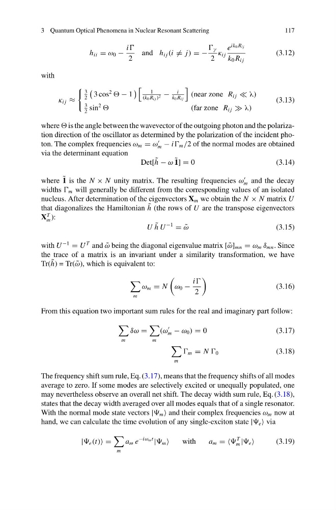
where is the angle between the wavevector of the outgoing photon and the polarization direction of the oscillator as determined by the polarization of the incident photon. The complex frequencies ω m = ω
m − i m /2 of the normal modes are obtained
via the determinant equation
Det[ ˜
h − ω ˜
1] = 0
(3.14)
where ˜
1 is the N × N unity matrix. The resulting frequencies ω
m and the decay
widths m will generally be different from the corresponding values of an isolated
nucleus. After determination of the eigenvectors X m we obtain the N × N matrix U
that diagonalizes the Hamiltonian ˜
h (the rows of U are the transpose eigenvectors
X
T
m ):
U ˜
h U
−1
= ˜
ω
(3.15)
with U
−1
= U
T and ˜
ω being the diagonal eigenvalue matrix [ ˜
ω] mn = ω m δ mn . Since
the trace of a matrix is an invariant under a similarity transformation, we have
Tr( ˜
h) = Tr( ˜
ω), which is equivalent to:
m
ω m = N
ω 0 −
i
2
(3.16)
From this equation two important sum rules for the real and imaginary part follow:
m
δω =
m
(ω
m − ω 0 ) = 0
(3.17)
m
m = N 0
(3.18)
The frequency shift sum rule, Eq. (3.17), means that the frequency shifts of all modes
average to zero. If some modes are selectively excited or unequally populated, one
may nevertheless observe an overall net shift. The decay width sum rule, Eq. (3.18),
states that the decay width averaged over all modes equals that of a single resonator.
With the normal mode state vectors | m and their complex frequencies ω m now at
hand, we can calculate the time evolution of any single-exciton state | e via
| e (t) =
m
a m e
−iω m t
| m
with
a m = =
T
m | e
(3.19)
117
h ii = ω 0 −
i
2
and h i j (i = j) = −
γ
2
κ i j
e
ik 0 R i j
k 0 R i j
(3.12)
with
κ i j ≈
3
2
3 cos
2
− 1
1
(k 0 R i j ) 2 −
i
k 0 R i j
(near zone R i j λ)
3
2
sin
2
( far zone R i j λ)
(3.13)
where is the angle between the wavevector of the outgoing photon and the polarization direction of the oscillator as determined by the polarization of the incident photon. The complex frequencies ω m = ω
m − i m /2 of the normal modes are obtained
via the determinant equation
Det[ ˜
h − ω ˜
1] = 0
(3.14)
where ˜
1 is the N × N unity matrix. The resulting frequencies ω
m and the decay
widths m will generally be different from the corresponding values of an isolated
nucleus. After determination of the eigenvectors X m we obtain the N × N matrix U
that diagonalizes the Hamiltonian ˜
h (the rows of U are the transpose eigenvectors
X
T
m ):
U ˜
h U
−1
= ˜
ω
(3.15)
with U
−1
= U
T and ˜
ω being the diagonal eigenvalue matrix [ ˜
ω] mn = ω m δ mn . Since
the trace of a matrix is an invariant under a similarity transformation, we have
Tr( ˜
h) = Tr( ˜
ω), which is equivalent to:
m
ω m = N
ω 0 −
i
2
(3.16)
From this equation two important sum rules for the real and imaginary part follow:
m
δω =
m
(ω
m − ω 0 ) = 0
(3.17)
m
m = N 0
(3.18)
The frequency shift sum rule, Eq. (3.17), means that the frequency shifts of all modes
average to zero. If some modes are selectively excited or unequally populated, one
may nevertheless observe an overall net shift. The decay width sum rule, Eq. (3.18),
states that the decay width averaged over all modes equals that of a single resonator.
With the normal mode state vectors | m and their complex frequencies ω m now at
hand, we can calculate the time evolution of any single-exciton state | e via
| e (t) =
m
a m e
−iω m t
| m
with
a m = =
T
m | e
(3.19)