

2 Synchrotron-Radiation-Based Energy-Domain Mössbauer …
95
The experimental time spectrum is written as ¯
I exp (q, t) = ¯
I (q, t) ⊗ D + B
discussed above.
From the definition of S cc (q, t), it follows that
S cc (q, t) =
1
ˆ
E 0 (0)
2
∞
−∞
∞
−∞
dt
dt
E 0
t
E
∗
0
t
g
q, t s + t
g
∗
q, t s + t + t
≡
∞
−∞
dt d I 0 (t d )S(q, t + t d )
(2.30)
where t d ≡ t
− t
. We define I 0 (t d ) ≡
∞
∫
−∞
dt
E
∗
0
t
E 0
t d + t
/
ˆ
E 0 (0)
2
. The
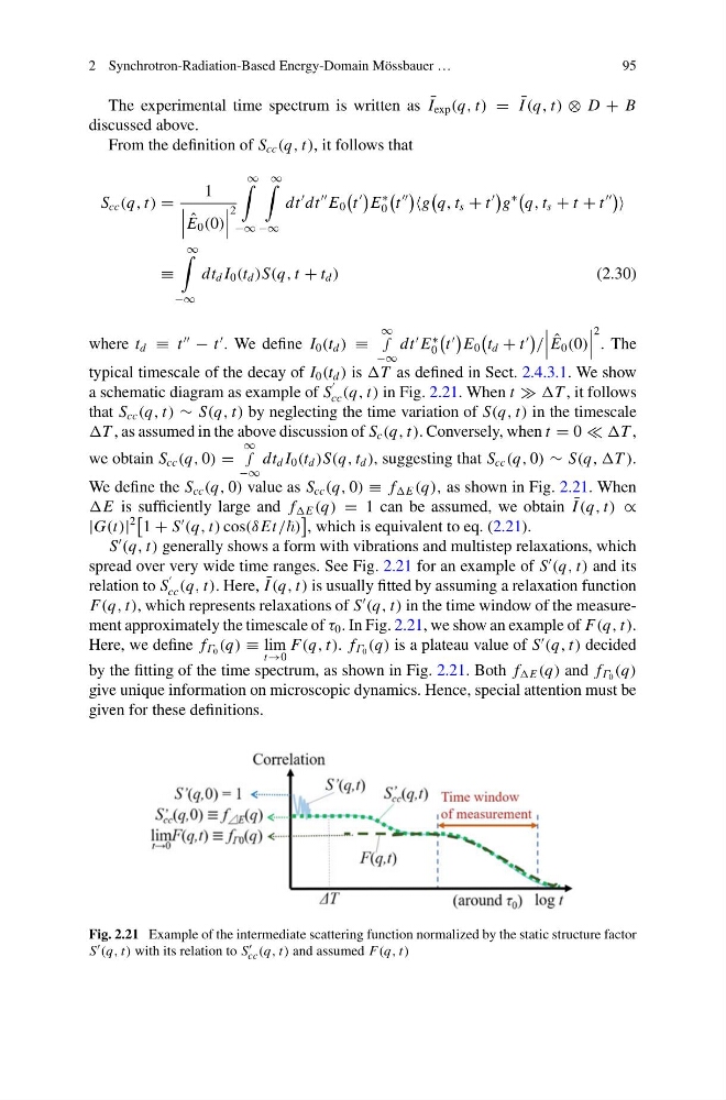
typical timescale of the decay of I 0 (t d ) is T as defined in Sect. 2.4.3.1. We show
a schematic diagram as example of S
cc (q, t) in Fig. 2.21. When t T , it follows
that S cc (q, t) ∼ S(q, t) by neglecting the time variation of S(q, t) in the timescale
T , as assumed in the above discussion of S c (q, t). Conversely, when t = 0 T ,
we obtain S cc (q, 0) =
∞
∫
−∞
dt d I 0 (t d )S(q, t d ), suggesting that S cc (q, 0) ∼ S(q, ,T ).
We define the S cc (q, 0) value as S cc (q, 0) ≡ f E (q), as shown in Fig. 2.21. When
E is sufficiently large and f E (q) = 1 can be assumed, we obtain ¯
I (q, t) ∝
|G(t)|
2
1 + S
(q, t) cos(δ Et/)
, which is equivalent to eq. (2.21).
S
(q, t) generally shows a form with vibrations and multistep relaxations, which
spread over very wide time ranges. See Fig. 2.21 for an example of S
(q, t) and its
relation to S
cc (q, t). Here, ¯
I (q, t) is usually fitted by assuming a relaxation function
F(q, t), which represents relaxations of S
(q, t) in the time window of the measurement approximately the timescale of τ 0 . In Fig. 2.21, we show an example of F(q, t).
Here, we define f Γ 0 (q) ≡ lim
t→0
F(q, t). f Γ 0 (q) is a plateau value of S
(q, t) decided
by the fitting of the time spectrum, as shown in Fig. 2.21. Both f E (q) and f Γ 0 (q)
give unique information on microscopic dynamics. Hence, special attention must be
given for these definitions.
Fig. 2.21 Example of the intermediate scattering function normalized by the static structure factor
S (q, t) with its relation to S
cc (q, t) and assumed F(q, t)
95
The experimental time spectrum is written as ¯
I exp (q, t) = ¯
I (q, t) ⊗ D + B
discussed above.
From the definition of S cc (q, t), it follows that
S cc (q, t) =
1
ˆ
E 0 (0)
2
∞
−∞
∞
−∞
dt
dt
E 0
t
E
∗
0
t
g
q, t s + t
g
∗
q, t s + t + t
≡
∞
−∞
dt d I 0 (t d )S(q, t + t d )
(2.30)
where t d ≡ t
− t
. We define I 0 (t d ) ≡
∞
∫
−∞
dt
E
∗
0
t
E 0
t d + t
/
ˆ
E 0 (0)
2
. The
typical timescale of the decay of I 0 (t d ) is T as defined in Sect. 2.4.3.1. We show
a schematic diagram as example of S
cc (q, t) in Fig. 2.21. When t T , it follows
that S cc (q, t) ∼ S(q, t) by neglecting the time variation of S(q, t) in the timescale
T , as assumed in the above discussion of S c (q, t). Conversely, when t = 0 T ,
we obtain S cc (q, 0) =
∞
∫
−∞
dt d I 0 (t d )S(q, t d ), suggesting that S cc (q, 0) ∼ S(q, ,T ).
We define the S cc (q, 0) value as S cc (q, 0) ≡ f E (q), as shown in Fig. 2.21. When
E is sufficiently large and f E (q) = 1 can be assumed, we obtain ¯
I (q, t) ∝
|G(t)|
2
1 + S
(q, t) cos(δ Et/)
, which is equivalent to eq. (2.21).
S
(q, t) generally shows a form with vibrations and multistep relaxations, which
spread over very wide time ranges. See Fig. 2.21 for an example of S
(q, t) and its
relation to S
cc (q, t). Here, ¯
I (q, t) is usually fitted by assuming a relaxation function
F(q, t), which represents relaxations of S
(q, t) in the time window of the measurement approximately the timescale of τ 0 . In Fig. 2.21, we show an example of F(q, t).
Here, we define f Γ 0 (q) ≡ lim
t→0
F(q, t). f Γ 0 (q) is a plateau value of S
(q, t) decided
by the fitting of the time spectrum, as shown in Fig. 2.21. Both f E (q) and f Γ 0 (q)
give unique information on microscopic dynamics. Hence, special attention must be
given for these definitions.
Fig. 2.21 Example of the intermediate scattering function normalized by the static structure factor
S (q, t) with its relation to S
cc (q, t) and assumed F(q, t)