

94
M. Seto et al.
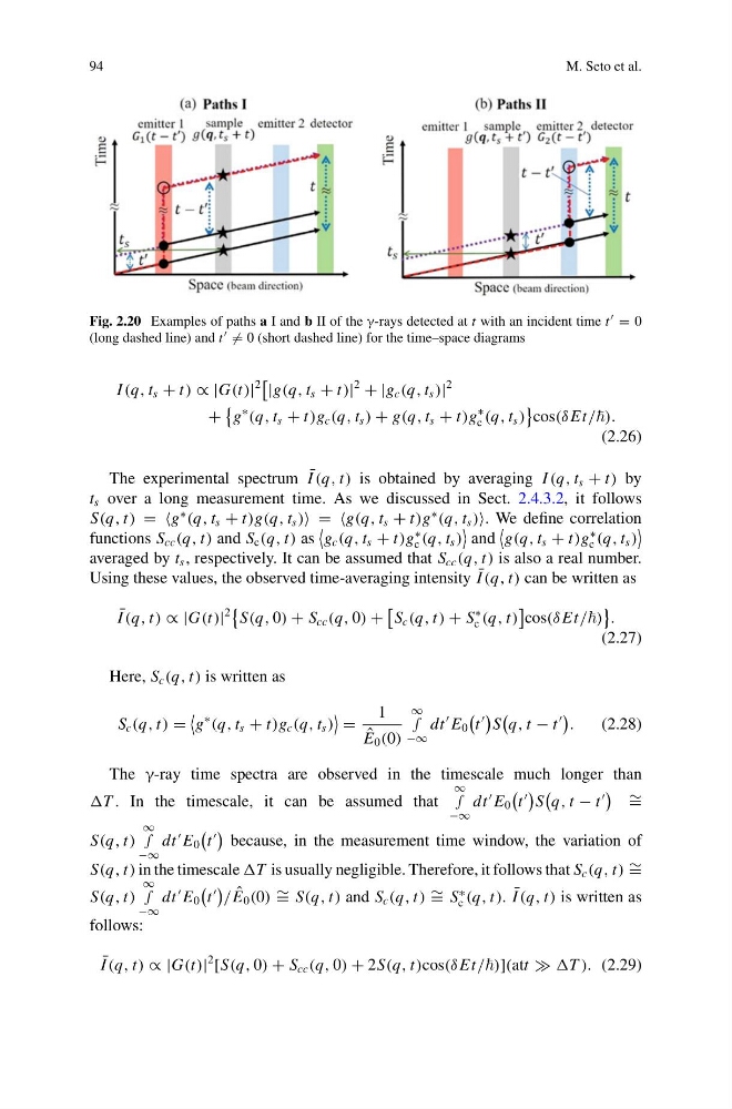
Fig. 2.20 Examples of paths a I and b II of the γ-rays detected at t with an incident time t = 0
(long dashed line) and t = 0 (short dashed line) for the time–space diagrams
I (q, t s + t) ∝ |G(t)|
2
|g(q, t s + t)|
2
+ |g c (q, t s )|
2
+
g
∗
(q, t s + t)g c (q, t s ) + g(q, t s + t)g
∗
c (q, t s )
cos(δ Et/).
(2.26)
The experimental spectrum ¯
I (q, t) is obtained by averaging I (q, t s + t) by
t s over a long measurement time. As we discussed in Sect. 2.4.3.2, it follows
S(q, t) = g
∗
(q, t s + t)g(q, t s ) = g(q, t s + t)g
∗
(q, t s ). We define correlation
functions S cc (q, t) and S c (q, t) as
g c (q, t s + t)g
∗
c (q, t s )
and
g(q, t s + t)g
∗
c (q, t s )
averaged by t s , respectively. It can be assumed that S cc (q, t) is also a real number.
Using these values, the observed time-averaging intensity ¯
I (q, t) can be written as
¯
I (q, t) ∝ |G(t)|
2
S(q, 0) + S cc (q, 0) +
S c (q, t) + S
∗
c (q, t)
cos(δ Et/)
.
(2.27)
Here, S c (q, t) is written as
S c (q, t) =
g
∗
(q, t s + t)g c (q, t s )
=
1
ˆ
E 0 (0)
∞
∫
−∞
dt
E 0
t
S
q, t − t
.
(2.28)
The γ-ray time spectra are observed in the timescale much longer than
T . In the timescale, it can be assumed that
∞
∫
−∞
dt
E 0
t
S
q, t − t
∼ =
S(q, t)
∞
∫
−∞
dt
E 0
t
because, in the measurement time window, the variation of
S(q, t) in the timescale T is usually negligible. Therefore, it follows that S c (q, t) ∼ =
S(q, t)
∞
∫
−∞
dt
E 0
t
/ ˆ
E 0 (0) ∼ = S(q, t) and S c (q, t) ∼ = S
∗
c (q, t). ¯
I (q, t) is written as
follows:
¯
I (q, t) ∝ |G(t)|
2 [S(q, 0) + S cc (q, 0) + 2S(q, t)cos(δ Et/)](att T ). (2.29)
M. Seto et al.
Fig. 2.20 Examples of paths a I and b II of the γ-rays detected at t with an incident time t = 0
(long dashed line) and t = 0 (short dashed line) for the time–space diagrams
I (q, t s + t) ∝ |G(t)|
2
|g(q, t s + t)|
2
+ |g c (q, t s )|
2
+
g
∗
(q, t s + t)g c (q, t s ) + g(q, t s + t)g
∗
c (q, t s )
cos(δ Et/).
(2.26)
The experimental spectrum ¯
I (q, t) is obtained by averaging I (q, t s + t) by
t s over a long measurement time. As we discussed in Sect. 2.4.3.2, it follows
S(q, t) = g
∗
(q, t s + t)g(q, t s ) = g(q, t s + t)g
∗
(q, t s ). We define correlation
functions S cc (q, t) and S c (q, t) as
g c (q, t s + t)g
∗
c (q, t s )
and
g(q, t s + t)g
∗
c (q, t s )
averaged by t s , respectively. It can be assumed that S cc (q, t) is also a real number.
Using these values, the observed time-averaging intensity ¯
I (q, t) can be written as
¯
I (q, t) ∝ |G(t)|
2
S(q, 0) + S cc (q, 0) +
S c (q, t) + S
∗
c (q, t)
cos(δ Et/)
.
(2.27)
Here, S c (q, t) is written as
S c (q, t) =
g
∗
(q, t s + t)g c (q, t s )
=
1
ˆ
E 0 (0)
∞
∫
−∞
dt
E 0
t
S
q, t − t
.
(2.28)
The γ-ray time spectra are observed in the timescale much longer than
T . In the timescale, it can be assumed that
∞
∫
−∞
dt
E 0
t
S
q, t − t
∼ =
S(q, t)
∞
∫
−∞
dt
E 0
t
because, in the measurement time window, the variation of
S(q, t) in the timescale T is usually negligible. Therefore, it follows that S c (q, t) ∼ =
S(q, t)
∞
∫
−∞
dt
E 0
t
/ ˆ
E 0 (0) ∼ = S(q, t) and S c (q, t) ∼ = S
∗
c (q, t). ¯
I (q, t) is written as
follows:
¯
I (q, t) ∝ |G(t)|
2 [S(q, 0) + S cc (q, 0) + 2S(q, t)cos(δ Et/)](att T ). (2.29)