

456
Y. Yoshida
∂G s (r, t)
∂t
=
1
τ
Z
j=1
1
Z
G s
r − R j , t
−
1
τ
G s (r, t),
(9.12)
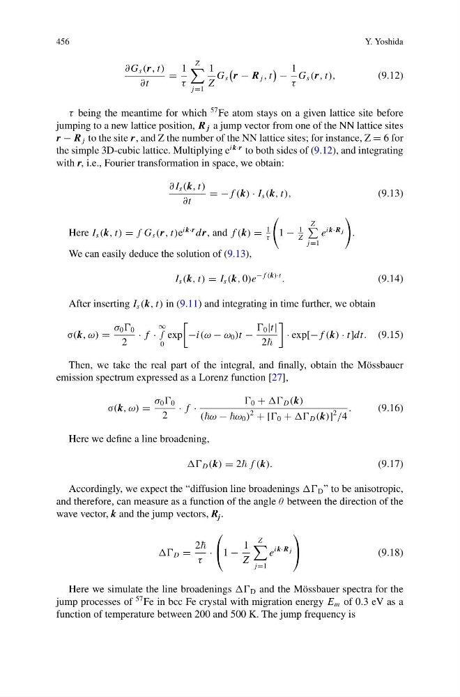
τ being the meantime for which
57 Fe atom stays on a given lattice site before
jumping to a new lattice position, R j a jump vector from one of the NN lattice sites
r − R j to the site r, and Z the number of the NN lattice sites; for instance, Z = 6 for
the simple 3D-cubic lattice. Multiplying e
i k·r to both sides of (9.12), and integrating
with r, i.e., Fourier transformation in space, we obtain:
∂ I s (k, t)
∂t
= − f (k) · I s (k, t),
(9.13)
Here I s (k, t) = ∫ G s (r, t)e
i k·r d r, and f (k) =
1
τ
1 −
1
Z
Z
j=1
e
i k·R j
.
We can easily deduce the solution of (9.13),
I s (k, t) = I s (k, 0)e
− f (k)·t
.
(9.14)
After inserting I s (k, t) in (9.11) and integrating in time further, we obtain
σ(k, ω) =
σ 0 0
2
· f ·
∞
∫
0
exp
−i(ω − ω 0 )t −
0 |t|
2
· exp[− f (k) · t]dt. (9.15)
Then, we take the real part of the integral, and finally, obtain the Mössbauer
emission spectrum expressed as a Lorenz function [27],
σ(k, ω) =
σ 0 0
2
· f ·
0 + D (k)
(ω − ω 0 )
2
+ [ 0 + D (k)]
2
/4
.
(9.16)
Here we define a line broadening,
D (k) = 2 f (k).
(9.17)
Accordingly, we expect the “diffusion line broadenings D ” to be anisotropic,
and therefore, can measure as a function of the angle θ between the direction of the
wave vector, k and the jump vectors, R j .
D =
2
τ
·
⎛
⎝ 1 −
1
Z
Z
j=1
e
i k·R j
⎞
⎠
(9.18)
Here we simulate the line broadenings D and the Mössbauer spectra for the
jump processes of
57 Fe in bcc Fe crystal with migration energy E m of 0.3 eV as a
function of temperature between 200 and 500 K. The jump frequency is
Y. Yoshida
∂G s (r, t)
∂t
=
1
τ
Z
j=1
1
Z
G s
r − R j , t
−
1
τ
G s (r, t),
(9.12)
τ being the meantime for which
57 Fe atom stays on a given lattice site before
jumping to a new lattice position, R j a jump vector from one of the NN lattice sites
r − R j to the site r, and Z the number of the NN lattice sites; for instance, Z = 6 for
the simple 3D-cubic lattice. Multiplying e
i k·r to both sides of (9.12), and integrating
with r, i.e., Fourier transformation in space, we obtain:
∂ I s (k, t)
∂t
= − f (k) · I s (k, t),
(9.13)
Here I s (k, t) = ∫ G s (r, t)e
i k·r d r, and f (k) =
1
τ
1 −
1
Z
Z
j=1
e
i k·R j
.
We can easily deduce the solution of (9.13),
I s (k, t) = I s (k, 0)e
− f (k)·t
.
(9.14)
After inserting I s (k, t) in (9.11) and integrating in time further, we obtain
σ(k, ω) =
σ 0 0
2
· f ·
∞
∫
0
exp
−i(ω − ω 0 )t −
0 |t|
2
· exp[− f (k) · t]dt. (9.15)
Then, we take the real part of the integral, and finally, obtain the Mössbauer
emission spectrum expressed as a Lorenz function [27],
σ(k, ω) =
σ 0 0
2
· f ·
0 + D (k)
(ω − ω 0 )
2
+ [ 0 + D (k)]
2
/4
.
(9.16)
Here we define a line broadening,
D (k) = 2 f (k).
(9.17)
Accordingly, we expect the “diffusion line broadenings D ” to be anisotropic,
and therefore, can measure as a function of the angle θ between the direction of the
wave vector, k and the jump vectors, R j .
D =
2
τ
·
⎛
⎝ 1 −
1
Z
Z
j=1
e
i k·R j
⎞
⎠
(9.18)
Here we simulate the line broadenings D and the Mössbauer spectra for the
jump processes of
57 Fe in bcc Fe crystal with migration energy E m of 0.3 eV as a
function of temperature between 200 and 500 K. The jump frequency is