

268
Y. Xu et al.
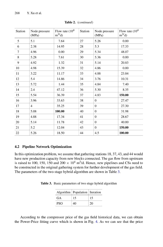
Table 2. (continued)
Station
Node pressure
(MPa)
Flow rate (10 4
m 3/ d)
Station
Node pressure
(MPa)
Flow rate (10 4
m 3/ d)
5
5.1
7.64
27
5.26
0.00
6
2.38
14.95
28
5.3
17.33
7
4.96
0.00
29
5.34
48.07
8
5.28
7.61
30
5.36
0.00
9
4.92
1.32
31
5.14
20.83
10
4.98
15.39
32
4.86
0.00
11
3.22
11.17
33
4.88
23.84
12
5.4
14.86
34
3.76
10.31
13
5.72
1.44
35
4.84
7.40
14
2.4
47.12
36
5.30
8.35
15
5.54
36.39
37
4.83
150.00
16
3.96
33.63
38
0
27.47
17
4
35.25
39
0
27.30
18
5.08
100.00
40
0
31.98
19
4.88
17.34
41
0
28.67
20
5.14
11.78
42
0
40.00
21
5.2
12.04
43
0
150.00
22
5.26
18.50
44
4.5
100.00
4.2 Pipeline Network Optimization
In this optimization problem, we assume that gathering stations 18, 37, 43, and 44 would
have new production capacity from new blocks connected. The gas flow from upstream
is raised to 100, 150, 150 and 200 × 10 4 m 3 /d. Hence, new pipelines and CSs need to
be constructed in the original gathering system for further development of the gas field.
The parameters of the two-stage hybrid algorithm are shown in Table 3.
Table 3. Basic parameters of two stage hybrid algorithm
Algorithm Population Iteration
GA
15
15
PSO
40
20
According to the compressor price of the gas field historical data, we can obtain
the Power-Price fitting curve which is shown in Fig. 4. As we can see that the price
Y. Xu et al.
Table 2. (continued)
Station
Node pressure
(MPa)
Flow rate (10 4
m 3/ d)
Station
Node pressure
(MPa)
Flow rate (10 4
m 3/ d)
5
5.1
7.64
27
5.26
0.00
6
2.38
14.95
28
5.3
17.33
7
4.96
0.00
29
5.34
48.07
8
5.28
7.61
30
5.36
0.00
9
4.92
1.32
31
5.14
20.83
10
4.98
15.39
32
4.86
0.00
11
3.22
11.17
33
4.88
23.84
12
5.4
14.86
34
3.76
10.31
13
5.72
1.44
35
4.84
7.40
14
2.4
47.12
36
5.30
8.35
15
5.54
36.39
37
4.83
150.00
16
3.96
33.63
38
0
27.47
17
4
35.25
39
0
27.30
18
5.08
100.00
40
0
31.98
19
4.88
17.34
41
0
28.67
20
5.14
11.78
42
0
40.00
21
5.2
12.04
43
0
150.00
22
5.26
18.50
44
4.5
100.00
4.2 Pipeline Network Optimization
In this optimization problem, we assume that gathering stations 18, 37, 43, and 44 would
have new production capacity from new blocks connected. The gas flow from upstream
is raised to 100, 150, 150 and 200 × 10 4 m 3 /d. Hence, new pipelines and CSs need to
be constructed in the original gathering system for further development of the gas field.
The parameters of the two-stage hybrid algorithm are shown in Table 3.
Table 3. Basic parameters of two stage hybrid algorithm
Algorithm Population Iteration
GA
15
15
PSO
40
20
According to the compressor price of the gas field historical data, we can obtain
the Power-Price fitting curve which is shown in Fig. 4. As we can see that the price