

Infrared Image Derivation Method for Generative Adversarial Network
241
blocks of fixed size N*N. This paper is based on the comparison and adjustment of the
data sets used in the experiment, taking N=60.
The algorithm generates an infrared image G(X, Z) under the constraint of the input
visible image X and the target segmentation map Z. During training, the original infrared
image Y is used as the reference image, and Z is obeying the target segmentation map
of visible. When the network training is set, the batch size is set to 1, and the network
structure parameters are updated every time a pair of images is input. The objective
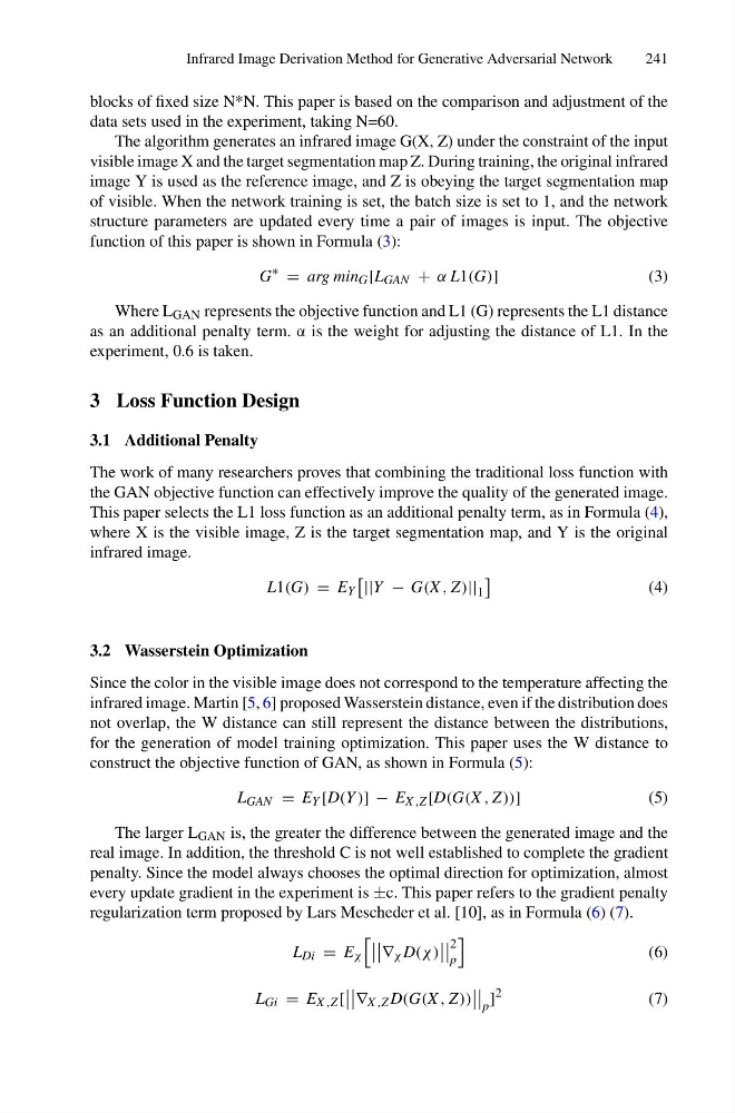
function of this paper is shown in Formula (3):
G
∗
= arg min G [L GAN + α L1(G)]
(3)
Where L GAN represents the objective function and L1 (G) represents the L1 distance
as an additional penalty term. α is the weight for adjusting the distance of L1. In the
experiment, 0.6 is taken.
3 Loss Function Design
3.1 Additional Penalty
The work of many researchers proves that combining the traditional loss function with
the GAN objective function can effectively improve the quality of the generated image.
This paper selects the L1 loss function as an additional penalty term, as in Formula (4),
where X is the visible image, Z is the target segmentation map, and Y is the original
infrared image.
L1(G) = E Y
||Y − G(X , Z)|| 1
(4)
3.2 Wasserstein Optimization
Since the color in the visible image does not correspond to the temperature affecting the
infrared image. Martin [5, 6] proposed Wasserstein distance, even if the distribution does
not overlap, the W distance can still represent the distance between the distributions,
for the generation of model training optimization. This paper uses the W distance to
construct the objective function of GAN, as shown in Formula (5):
L GAN = E Y [D(Y )] − E X ,Z [D(G(X , Z))]
(5)
The larger L GAN is, the greater the difference between the generated image and the
real image. In addition, the threshold C is not well established to complete the gradient
penalty. Since the model always chooses the optimal direction for optimization, almost
every update gradient in the experiment is ±c. This paper refers to the gradient penalty
regularization term proposed by Lars Mescheder et al. [10], as in Formula (6) (7).
L Di = E χ
∇ χ D(χ )
2
p
(6)
L Gi = E X ,Z [
∇ X ,Z D(G(X , Z))
p
]
2
(7)
241
blocks of fixed size N*N. This paper is based on the comparison and adjustment of the
data sets used in the experiment, taking N=60.
The algorithm generates an infrared image G(X, Z) under the constraint of the input
visible image X and the target segmentation map Z. During training, the original infrared
image Y is used as the reference image, and Z is obeying the target segmentation map
of visible. When the network training is set, the batch size is set to 1, and the network
structure parameters are updated every time a pair of images is input. The objective
function of this paper is shown in Formula (3):
G
∗
= arg min G [L GAN + α L1(G)]
(3)
Where L GAN represents the objective function and L1 (G) represents the L1 distance
as an additional penalty term. α is the weight for adjusting the distance of L1. In the
experiment, 0.6 is taken.
3 Loss Function Design
3.1 Additional Penalty
The work of many researchers proves that combining the traditional loss function with
the GAN objective function can effectively improve the quality of the generated image.
This paper selects the L1 loss function as an additional penalty term, as in Formula (4),
where X is the visible image, Z is the target segmentation map, and Y is the original
infrared image.
L1(G) = E Y
||Y − G(X , Z)|| 1
(4)
3.2 Wasserstein Optimization
Since the color in the visible image does not correspond to the temperature affecting the
infrared image. Martin [5, 6] proposed Wasserstein distance, even if the distribution does
not overlap, the W distance can still represent the distance between the distributions,
for the generation of model training optimization. This paper uses the W distance to
construct the objective function of GAN, as shown in Formula (5):
L GAN = E Y [D(Y )] − E X ,Z [D(G(X , Z))]
(5)
The larger L GAN is, the greater the difference between the generated image and the
real image. In addition, the threshold C is not well established to complete the gradient
penalty. Since the model always chooses the optimal direction for optimization, almost
every update gradient in the experiment is ±c. This paper refers to the gradient penalty
regularization term proposed by Lars Mescheder et al. [10], as in Formula (6) (7).
L Di = E χ
∇ χ D(χ )
2
p
(6)
L Gi = E X ,Z [
∇ X ,Z D(G(X , Z))
p
]
2
(7)