

68
E. V. Chimanski et al.
Exp(E) = e 0 exp
(E − E 0 )
β
.
(4)
The widths σ, γ , and β of the distributions are taken to represent the p-h mixing
caused by the residual interaction. Their mean energy values E 0 are close to the
energy of the mode that most contributes to the state.
2.2 Simplified Particle–Hole Basis
The calculation of the p-h transition matrix elements using the single particle states
from the Hartree–Fock (HF) solutions can be very time consuming due to the slow
convergence of the mean field. As a first approximation we use a simplified model
based on quantum harmonic oscillator (QHO) functions. Our work is reduced to
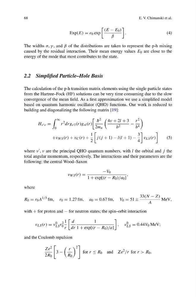
building and diagonalizing the following matrix [19]:
H ν ν =
∞
0
r
2 drg ν l (r)g νl (r)
¯
h 2
2m n
4ν + 2l + 3
b 2
−
r 2
b 4
+v W S (r) + v C (r) +
1
2
j (j + 1) − l(l + 1) −
3
4
v LS (r)
(5)
where ν , ν are the principal QHO quantum numbers, with l the orbital and j the
total angular momentum, respectively. The interactions and their parameters are the
following: the central Wood–Saxon
v W S (r) =
−V 0
1 + exp[(r − R 0 )/a 0 ]
,
where
R 0 = r 0 A
1/3 fm, r 0 = 1.27 fm, a 0 = 0.67 fm, V 0 = 51 ±
33(N − Z)
A
MeV,
with + for proton and − for neutron states; the spin–orbit interaction
v LS (r) = v
0
LS r
2
0
1
r
d
dr
1
1 + exp[(r − R 0 )/a]
, v
0
LS = 0.44V 0 MeV;
and the Coulomb repulsion
Ze 2
2R 0
3 −
r
R 0
2
for r ≤ R 0 and Ze
2 /r for r > R 0 .
E. V. Chimanski et al.
Exp(E) = e 0 exp
(E − E 0 )
β
.
(4)
The widths σ, γ , and β of the distributions are taken to represent the p-h mixing
caused by the residual interaction. Their mean energy values E 0 are close to the
energy of the mode that most contributes to the state.
2.2 Simplified Particle–Hole Basis
The calculation of the p-h transition matrix elements using the single particle states
from the Hartree–Fock (HF) solutions can be very time consuming due to the slow
convergence of the mean field. As a first approximation we use a simplified model
based on quantum harmonic oscillator (QHO) functions. Our work is reduced to
building and diagonalizing the following matrix [19]:
H ν ν =
∞
0
r
2 drg ν l (r)g νl (r)
¯
h 2
2m n
4ν + 2l + 3
b 2
−
r 2
b 4
+v W S (r) + v C (r) +
1
2
j (j + 1) − l(l + 1) −
3
4
v LS (r)
(5)
where ν , ν are the principal QHO quantum numbers, with l the orbital and j the
total angular momentum, respectively. The interactions and their parameters are the
following: the central Wood–Saxon
v W S (r) =
−V 0
1 + exp[(r − R 0 )/a 0 ]
,
where
R 0 = r 0 A
1/3 fm, r 0 = 1.27 fm, a 0 = 0.67 fm, V 0 = 51 ±
33(N − Z)
A
MeV,
with + for proton and − for neutron states; the spin–orbit interaction
v LS (r) = v
0
LS r
2
0
1
r
d
dr
1
1 + exp[(r − R 0 )/a]
, v
0
LS = 0.44V 0 MeV;
and the Coulomb repulsion
Ze 2
2R 0
3 −
r
R 0
2
for r ≤ R 0 and Ze
2 /r for r > R 0 .