

108
Y. Alhassid
10
0
10
4
10
8
10
12
10
16
10
20
0
10
20
30
40
50
ρ (MeV
-1
)
E x (MeV)
10
0
10
4
10
8
0
2
4
6
8
ρ (MeV
-1
)
E x (MeV)
Fig. 4 State density of 162 Dy vs. excitation energy E x . The AFMC state density (solid circles) is
compared with the HF density (solid line). The inset shows the low excitation energy region. Taken
from Ref. [49]
0
2
4
6
8
0
0.01
0.02
0.03
0.04
ρ
J
/ρ
σ
2 = 7.92
σ
2 = 10.4
0
2
4
6
8
J
σ
2 = 7.96
σ
2 = 10.9
0
2
4
6
8
σ
2 = 8.11
σ
2 = 11.8
56
Fe
55
Fe
60
Co
E x = 4.39 MeV
E x = 5.6 MeV
E x = 3.39 MeV
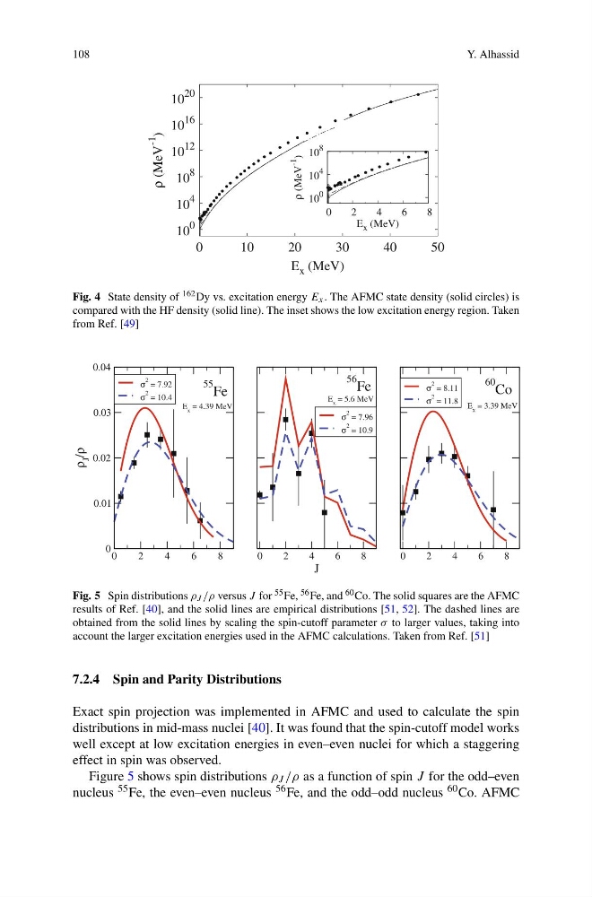
Fig. 5 Spin distributions ρ J /ρ versus J for 55 Fe, 56 Fe, and 60 Co. The solid squares are the AFMC
results of Ref. [40], and the solid lines are empirical distributions [51, 52]. The dashed lines are
obtained from the solid lines by scaling the spin-cutoff parameter σ to larger values, taking into
account the larger excitation energies used in the AFMC calculations. Taken from Ref. [51]
7.2.4 Spin and Parity Distributions
Exact spin projection was implemented in AFMC and used to calculate the spin
distributions in mid-mass nuclei [40]. It was found that the spin-cutoff model works
well except at low excitation energies in even–even nuclei for which a staggering
effect in spin was observed.
Figure 5 shows spin distributions ρ J /ρ as a function of spin J for the odd–even
nucleus 55 Fe, the even–even nucleus 56 Fe, and the odd–odd nucleus 60 Co. AFMC
Y. Alhassid
10
0
10
4
10
8
10
12
10
16
10
20
0
10
20
30
40
50
ρ (MeV
-1
)
E x (MeV)
10
0
10
4
10
8
0
2
4
6
8
ρ (MeV
-1
)
E x (MeV)
Fig. 4 State density of 162 Dy vs. excitation energy E x . The AFMC state density (solid circles) is
compared with the HF density (solid line). The inset shows the low excitation energy region. Taken
from Ref. [49]
0
2
4
6
8
0
0.01
0.02
0.03
0.04
ρ
J
/ρ
σ
2 = 7.92
σ
2 = 10.4
0
2
4
6
8
J
σ
2 = 7.96
σ
2 = 10.9
0
2
4
6
8
σ
2 = 8.11
σ
2 = 11.8
56
Fe
55
Fe
60
Co
E x = 4.39 MeV
E x = 5.6 MeV
E x = 3.39 MeV
Fig. 5 Spin distributions ρ J /ρ versus J for 55 Fe, 56 Fe, and 60 Co. The solid squares are the AFMC
results of Ref. [40], and the solid lines are empirical distributions [51, 52]. The dashed lines are
obtained from the solid lines by scaling the spin-cutoff parameter σ to larger values, taking into
account the larger excitation energies used in the AFMC calculations. Taken from Ref. [51]
7.2.4 Spin and Parity Distributions
Exact spin projection was implemented in AFMC and used to calculate the spin
distributions in mid-mass nuclei [40]. It was found that the spin-cutoff model works
well except at low excitation energies in even–even nuclei for which a staggering
effect in spin was observed.
Figure 5 shows spin distributions ρ J /ρ as a function of spin J for the odd–even
nucleus 55 Fe, the even–even nucleus 56 Fe, and the odd–odd nucleus 60 Co. AFMC