

624
V. Skorych et al.
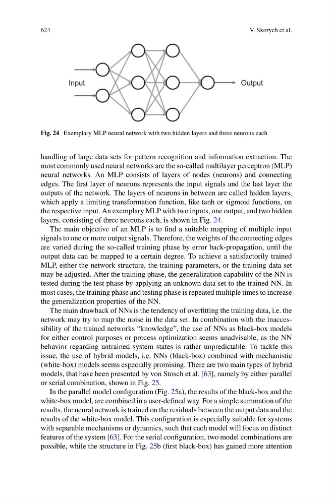
Fig. 24 Exemplary MLP neural network with two hidden layers and three neurons each
handling of large data sets for pattern recognition and information extraction. The
most commonly used neural networks are the so-called multilayer perceptron (MLP)
neural networks. An MLP consists of layers of nodes (neurons) and connecting
edges. The first layer of neurons represents the input signals and the last layer the
outputs of the network. The layers of neurons in between are called hidden layers,
which apply a limiting transformation function, like tanh or sigmoid functions, on
the respective input. An exemplary MLP with two inputs, one output, and two hidden
layers, consisting of three neurons each, is shown in Fig. 24.
The main objective of an MLP is to find a suitable mapping of multiple input
signals to one or more output signals. Therefore, the weights of the connecting edges
are varied during the so-called training phase by error back-propagation, until the
output data can be mapped to a certain degree. To achieve a satisfactorily trained
MLP, either the network structure, the training parameters, or the training data set
may be adjusted. After the training phase, the generalization capability of the NN is
tested during the test phase by applying an unknown data set to the trained NN. In
most cases, the training phase and testing phase is repeated multiple times to increase
the generalization properties of the NN.
The main drawback of NNs is the tendency of overfitting the training data, i.e. the
network may try to map the noise in the data set. In combination with the inaccessibility of the trained networks “knowledge”, the use of NNs as black-box models
for either control purposes or process optimization seems unadvisable, as the NN
behavior regarding untrained system states is rather unpredictable. To tackle this
issue, the use of hybrid models, i.e. NNs (black-box) combined with mechanistic
(white-box) models seems especially promising. There are two main types of hybrid
models, that have been presented by von Stosch et al. [63], namely by either parallel
or serial combination, shown in Fig. 25.
In the parallel model configuration (Fig. 25a), the results of the black-box and the
white-box model, are combined in a user-defined way. For a simple summation of the
results, the neural network is trained on the residuals between the output data and the
results of the white-box model. This configuration is especially suitable for systems
with separable mechanisms or dynamics, such that each model will focus on distinct
features of the system [63]. For the serial configuration, two model combinations are
possible, while the structure in Fig. 25b (first black-box) has gained more attention