

17 A Framework for Dynamic Simulation of Interconnected …
613
milling of the particles occurs. As a result, the proportion of wet material in the fine
fraction increases.
In [52], new approaches for calculating transformation matrices from the population balance equations for agglomeration and milling have been developed. The
finite volume method for spatial discretization and the second-order Runge-Kutta
method for obtaining the complete discretized form of the PBE were applied to
derive transformation laws.
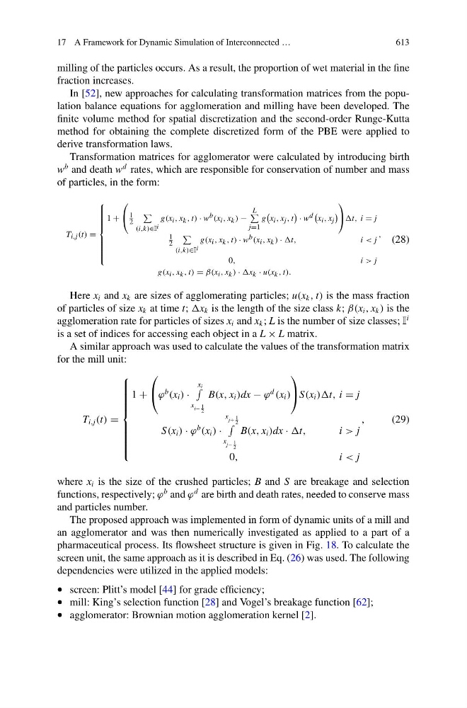
Transformation matrices for agglomerator were calculated by introducing birth
w
b and death w
d rates, which are responsible for conservation of number and mass
of particles, in the form:
T i,j (t) =
⎧
⎪ ⎪ ⎪ ⎪ ⎪ ⎪ ⎨
⎪ ⎪ ⎪ ⎪ ⎪ ⎪ ⎩
1 +
⎛
⎝ 1
2
(i,k)∈I i
g(x i , x k , t) · w b (x i , x k ) −
L
j=1
g
x i , x j , t
· w d
x i , x j
⎞
⎠ t, i = j
1
2
(i,k)∈I i
g(x i , x k , t) · w b (x i , x k ) · t,
i < j
0,
i > j
,
g(x i , x k , t) = β(x i , x k ) · x k · u(x k , t).
(28)
Here x i and x k are sizes of agglomerating particles; u(x k , t) is the mass fraction
of particles of size x k at time t; x k is the length of the size class k; β(x i , x k ) is the
agglomeration rate for particles of sizes x i and x k ; L is the number of size classes; I
i
is a set of indices for accessing each object in a L × L matrix.
A similar approach was used to calculate the values of the transformation matrix
for the mill unit:
T i,j (t) =
⎧
⎪ ⎪ ⎪ ⎪ ⎪ ⎪ ⎪ ⎨
⎪ ⎪ ⎪ ⎪ ⎪ ⎪ ⎪ ⎩
1 +
⎛
⎝ ϕ
b
(x i ) ·
x i
x i− 1
2
B(x, x i )dx − ϕ
d
(x i )
⎞
⎠ S(x i )t, i = j
S(x i ) · ϕ
b
(x i ) ·
x j+ 1
2
x j− 1
2
B(x, x i )dx · t,
i > j
0,
i < j
,
(29)
where x i is the size of the crushed particles; B and S are breakage and selection
functions, respectively; ϕ
b and ϕ
d are birth and death rates, needed to conserve mass
and particles number.
The proposed approach was implemented in form of dynamic units of a mill and
an agglomerator and was then numerically investigated as applied to a part of a
pharmaceutical process. Its flowsheet structure is given in Fig. 18. To calculate the
screen unit, the same approach as it is described in Eq. (26) was used. The following
dependencies were utilized in the applied models:
• screen: Plitt’s model [44] for grade efficiency;
• mill: King’s selection function [28] and Vogel’s breakage function [62];
• agglomerator: Brownian motion agglomeration kernel [2].