

600
V. Skorych et al.
since some types of equations are more common in models, several solvers were
integrated into the modelling framework to facilitate the addition of new units to the
system.
4.1 Solver of Differential-Algebraic Equations
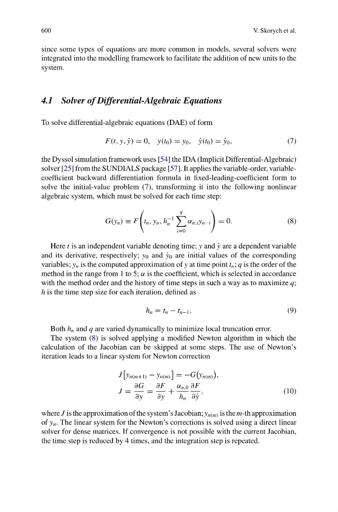
To solve differential-algebraic equations (DAE) of form
F(t, y, ˙
y) = 0, y(t 0 ) = y 0 , ˙
y(t 0 ) = ˙
y 0 ,
(7)
the Dyssol simulation framework uses [54] the IDA (Implicit Differential-Algebraic)
solver [25] from the SUNDIALS package [57]. It applies the variable-order, variablecoefficient backward differentiation formula in fixed-leading-coefficient form to
solve the initial-value problem (7), transforming it into the following nonlinear
algebraic system, which must be solved for each time step:
G(y n ) ≡ F
t n , y n , h
−1
n
q
i=0
α n,i y n−i
= 0.
(8)
Here t is an independent variable denoting time; y and ˙
y are a dependent variable
and its derivative, respectively; y 0 and ˙
y 0 are initial values of the corresponding
variables; y n is the computed approximation of y at time point t n ; q is the order of the
method in the range from 1 to 5; α is the coefficient, which is selected in accordance
with the method order and the history of time steps in such a way as to maximize q;
h is the time step size for each iteration, defined as
h n = t n − t n−1 .
(9)
Both h n and q are varied dynamically to minimize local truncation error.
The system (8) is solved applying a modified Newton algorithm in which the
calculation of the Jacobian can be skipped at some steps. The use of Newton’s
iteration leads to a linear system for Newton correction
J
y n(m+1) − y n(m)
= −G
y n(m)
,
J =
∂G
∂y
=
∂F
∂y
+
α n,0
h n
∂F
∂ ˙
y
,
(10)
where J is the approximation of the system’s Jacobian; y n(m) is the m-th approximation
of y n . The linear system for the Newton’s corrections is solved using a direct linear
solver for dense matrices. If convergence is not possible with the current Jacobian,
the time step is reduced by 4 times, and the integration step is repeated.
V. Skorych et al.
since some types of equations are more common in models, several solvers were
integrated into the modelling framework to facilitate the addition of new units to the
system.
4.1 Solver of Differential-Algebraic Equations
To solve differential-algebraic equations (DAE) of form
F(t, y, ˙
y) = 0, y(t 0 ) = y 0 , ˙
y(t 0 ) = ˙
y 0 ,
(7)
the Dyssol simulation framework uses [54] the IDA (Implicit Differential-Algebraic)
solver [25] from the SUNDIALS package [57]. It applies the variable-order, variablecoefficient backward differentiation formula in fixed-leading-coefficient form to
solve the initial-value problem (7), transforming it into the following nonlinear
algebraic system, which must be solved for each time step:
G(y n ) ≡ F
t n , y n , h
−1
n
q
i=0
α n,i y n−i
= 0.
(8)
Here t is an independent variable denoting time; y and ˙
y are a dependent variable
and its derivative, respectively; y 0 and ˙
y 0 are initial values of the corresponding
variables; y n is the computed approximation of y at time point t n ; q is the order of the
method in the range from 1 to 5; α is the coefficient, which is selected in accordance
with the method order and the history of time steps in such a way as to maximize q;
h is the time step size for each iteration, defined as
h n = t n − t n−1 .
(9)
Both h n and q are varied dynamically to minimize local truncation error.
The system (8) is solved applying a modified Newton algorithm in which the
calculation of the Jacobian can be skipped at some steps. The use of Newton’s
iteration leads to a linear system for Newton correction
J
y n(m+1) − y n(m)
= −G
y n(m)
,
J =
∂G
∂y
=
∂F
∂y
+
α n,0
h n
∂F
∂ ˙
y
,
(10)
where J is the approximation of the system’s Jacobian; y n(m) is the m-th approximation
of y n . The linear system for the Newton’s corrections is solved using a direct linear
solver for dense matrices. If convergence is not possible with the current Jacobian,
the time step is reduced by 4 times, and the integration step is repeated.