

16 Modeling, Simulation and Optimization of Process Chains
571
min
P
−E[q tot ] + 10
−2
L 1 ((0,t f )) + 10
−2
˙
P
2
L 2 ((0,t f )) s.t.
q t (t, x) + ∂ x
100
100+W q (t)
q(t, x)
= 0.1
(1 − 1 (x))(1 − 2 (x)) − 1
q(t, x)
+ q crush (P(t), t, x)
q(0, x) = q 0 (x)
W q (t) =
∞
x min
4π y
2 q(t, y) dy
P(t) ∈ [0, 100]
Where it was used that a term maximizing a property also minimizes the sign changed
property, and vice versa. After having stated the mathematical model of the here
considered issue, the corresponding numerical results out of the optimization will be
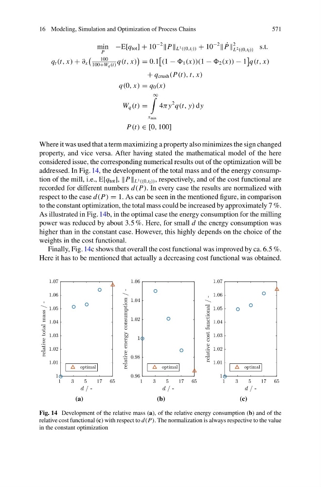
addressed. In Fig. 14, the development of the total mass and of the energy consumption of the mill, i.e., E[q tot ], L 1 ((0,t f )) , respectively, and of the cost functional are
recorded for different numbers d(P). In every case the results are normalized with
respect to the case d(P) = 1. As can be seen in the mentioned figure, in comparison
to the constant optimization, the total mass could be increased by approximately 7 %.
As illustrated in Fig. 14b, in the optimal case the energy consumption for the milling
power was reduced by about 3.5 %. Here, for small d the energy consumption was
higher than in the constant case. However, this highly depends on the choice of the
weights in the cost functional.
Finally, Fig. 14c shows that overall the cost functional was improved by ca. 6.5 %.
Here it has to be mentioned that actually a decreasing cost functional was obtained.
Fig. 14 Development of the relative mass (a), of the relative energy consumption (b) and of the
relative cost functional (c) with respect to d(P). The normalization is always respective to the value
in the constant optimization
571
min
P
−E[q tot ] + 10
−2
L 1 ((0,t f )) + 10
−2
˙
P
2
L 2 ((0,t f )) s.t.
q t (t, x) + ∂ x
100
100+W q (t)
q(t, x)
= 0.1
(1 − 1 (x))(1 − 2 (x)) − 1
q(t, x)
+ q crush (P(t), t, x)
q(0, x) = q 0 (x)
W q (t) =
∞
x min
4π y
2 q(t, y) dy
P(t) ∈ [0, 100]
Where it was used that a term maximizing a property also minimizes the sign changed
property, and vice versa. After having stated the mathematical model of the here
considered issue, the corresponding numerical results out of the optimization will be
addressed. In Fig. 14, the development of the total mass and of the energy consumption of the mill, i.e., E[q tot ], L 1 ((0,t f )) , respectively, and of the cost functional are
recorded for different numbers d(P). In every case the results are normalized with
respect to the case d(P) = 1. As can be seen in the mentioned figure, in comparison
to the constant optimization, the total mass could be increased by approximately 7 %.
As illustrated in Fig. 14b, in the optimal case the energy consumption for the milling
power was reduced by about 3.5 %. Here, for small d the energy consumption was
higher than in the constant case. However, this highly depends on the choice of the
weights in the cost functional.
Finally, Fig. 14c shows that overall the cost functional was improved by ca. 6.5 %.
Here it has to be mentioned that actually a decreasing cost functional was obtained.
Fig. 14 Development of the relative mass (a), of the relative energy consumption (b) and of the
relative cost functional (c) with respect to d(P). The normalization is always respective to the value
in the constant optimization