

16 Modeling, Simulation and Optimization of Process Chains
567
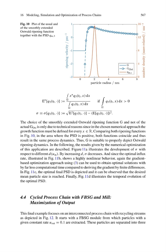
Fig. 10 Plot of the usual and
of the smoothly extended
Ostwald ripening function
together with the PSD q in,3
E
n
[q 3 (t f , ·)] :=
x
n q 3 (t f , x) dx
q 3 (t f , x) dx
if
q 3 (t f , x) dx > 0
σ ≡ σ [q 3 (t f , ·)] :=
E 2 [q 3 (t f , ·)] − (E[q 3 (t f , ·)]) 2 .
The choice of the smoothly extended Ostwald ripening function G and not of the
actual G Ost is only due to technical reasons since in the chosen numerical approach the
growth function must be defined for every x ∈ R. Comparing both ripening functions
in Fig. 10, in the area where the PSD is positive, both functions coincide and thus
result in the same process dynamics. Thus, G is suitable to properly depict Ostwald
ripening dynamics. In the following, the results given by the numerical optimization
of this application are described. Figure 11a illustrates the development of σ with
respect to different d(u in ). By increasing d, σ decreases. And since the optimal influx
rate, illustrated in Fig. 11b, shows a highly nonlinear behavior, again the gradientbased optimization approach using (3) can be used to obtain optimal solutions with
by far less computational time compared to deriving the gradient by finite differences.
In Fig. 11c, the optimal final PSD is depicted and it can be observed that the desired
mean particle size is reached. Finally, Fig. 11d illustrates the temporal evolution of
the optimal PSD.
4.4 Cycled Process Chain with FBSG and Mill:
Maximization of Output
This final example focuses on an interconnected process chain with recycling streams
as depicted in Fig. 12. It starts with a FBSG module from which particles with a
given constant rate u out ≡ 0.1 are extracted. These particles are separated into three
567
Fig. 10 Plot of the usual and
of the smoothly extended
Ostwald ripening function
together with the PSD q in,3
E
n
[q 3 (t f , ·)] :=
x
n q 3 (t f , x) dx
q 3 (t f , x) dx
if
q 3 (t f , x) dx > 0
σ ≡ σ [q 3 (t f , ·)] :=
E 2 [q 3 (t f , ·)] − (E[q 3 (t f , ·)]) 2 .
The choice of the smoothly extended Ostwald ripening function G and not of the
actual G Ost is only due to technical reasons since in the chosen numerical approach the
growth function must be defined for every x ∈ R. Comparing both ripening functions
in Fig. 10, in the area where the PSD is positive, both functions coincide and thus
result in the same process dynamics. Thus, G is suitable to properly depict Ostwald
ripening dynamics. In the following, the results given by the numerical optimization
of this application are described. Figure 11a illustrates the development of σ with
respect to different d(u in ). By increasing d, σ decreases. And since the optimal influx
rate, illustrated in Fig. 11b, shows a highly nonlinear behavior, again the gradientbased optimization approach using (3) can be used to obtain optimal solutions with
by far less computational time compared to deriving the gradient by finite differences.
In Fig. 11c, the optimal final PSD is depicted and it can be observed that the desired
mean particle size is reached. Finally, Fig. 11d illustrates the temporal evolution of
the optimal PSD.
4.4 Cycled Process Chain with FBSG and Mill:
Maximization of Output
This final example focuses on an interconnected process chain with recycling streams
as depicted in Fig. 12. It starts with a FBSG module from which particles with a
given constant rate u out ≡ 0.1 are extracted. These particles are separated into three