

542
G. Kotalczyk and F. E. Kruis
dn S (v, t)
dt
= + f F2→S · n F2 (v, t) − f S→F · n M (v, t) + F D→S · n D (v, t)
dn F1 (v, t)
dt
= + f S→F · n S (v, t) · S sep (v)
dn F2 (v, t)
dt
= + f S→F · n S (v, t) · (1 − S sep (v)) − f F2→S · n F2 (v, t)
(17)
The explicit particle exchange rates for these equations are summarized in Table 4.
The following form of the separation function S sep (v) has been used for the screen:
S sep (v) =
⎧
⎨
⎩
1,
v > v
sep
max
(v − v
sep
min )/(v
sep
max − v
sep
min ), v
sep
max > v > v
sep
min
0,
v
sep
min > v
(18)
The separation cut-off values v
sep
max = π(d
sep
max )
3
/6 and v
sep
min = π(d
sep
max )
3
/6
correspond to the diameters d
sep
max = 57 nm and d
sep
min = 40 nm.
As initial conditions for the PSDs in the mixer n
0
M (v) (resp. screen n
0
S (v)), two
identic log-normal distributions with a geometric mean diameter of 50 nm, a geometric standard deviation of 1.2 and a total number-concentration of 10
10 m
−3 have
been used. The same distribution has been used as feed PSD, i.e. n D (v). Both filters
are empty at the beginning of the simulation (n
0
F1 (v) = n
0
F2 (v) = 0).
A fixed pivot method [58] has been used as benchmark. The continuous initial
PSDs are thereby discretized with the help of a geometric grid of 1000 pivot points,
covering a particle size range from 1 nm to 10 μm. In the scope of this approach,
the set of Eqs. (16) or (17) is interpreted as the rate of change for each single pivot
point with its respective volume v.
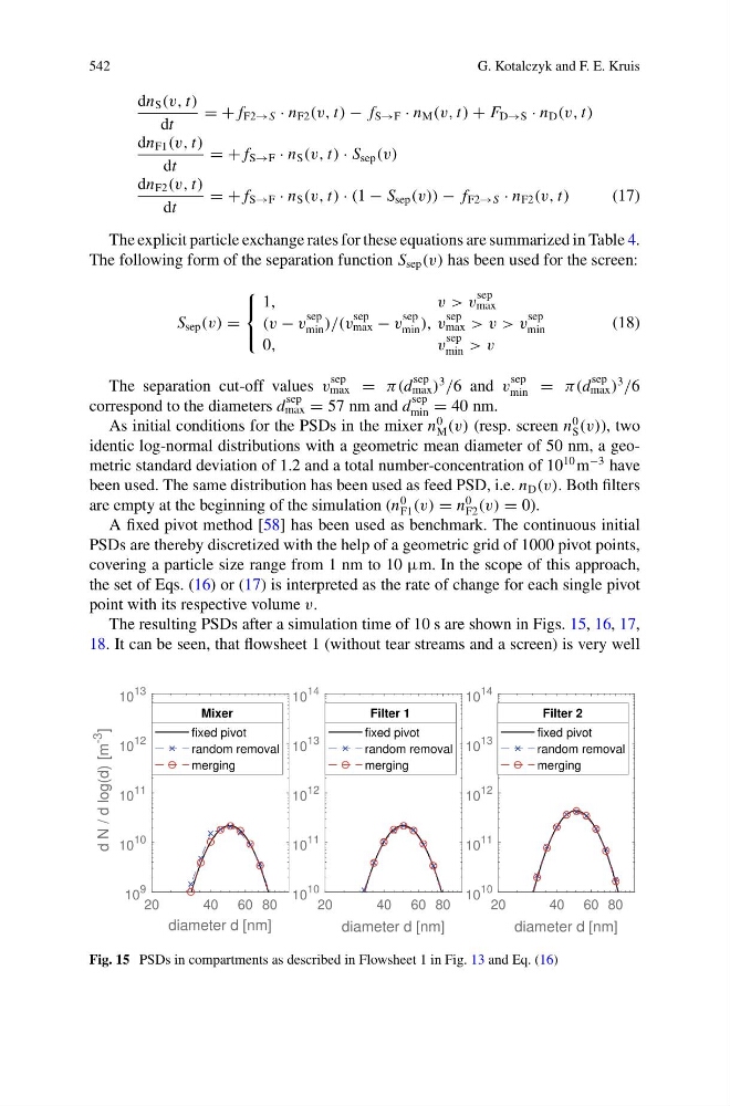
The resulting PSDs after a simulation time of 10 s are shown in Figs. 15, 16, 17,
18. It can be seen, that flowsheet 1 (without tear streams and a screen) is very well
Fig. 15 PSDs in compartments as described in Flowsheet 1 in Fig. 13 and Eq. (16)
G. Kotalczyk and F. E. Kruis
dn S (v, t)
dt
= + f F2→S · n F2 (v, t) − f S→F · n M (v, t) + F D→S · n D (v, t)
dn F1 (v, t)
dt
= + f S→F · n S (v, t) · S sep (v)
dn F2 (v, t)
dt
= + f S→F · n S (v, t) · (1 − S sep (v)) − f F2→S · n F2 (v, t)
(17)
The explicit particle exchange rates for these equations are summarized in Table 4.
The following form of the separation function S sep (v) has been used for the screen:
S sep (v) =
⎧
⎨
⎩
1,
v > v
sep
max
(v − v
sep
min )/(v
sep
max − v
sep
min ), v
sep
max > v > v
sep
min
0,
v
sep
min > v
(18)
The separation cut-off values v
sep
max = π(d
sep
max )
3
/6 and v
sep
min = π(d
sep
max )
3
/6
correspond to the diameters d
sep
max = 57 nm and d
sep
min = 40 nm.
As initial conditions for the PSDs in the mixer n
0
M (v) (resp. screen n
0
S (v)), two
identic log-normal distributions with a geometric mean diameter of 50 nm, a geometric standard deviation of 1.2 and a total number-concentration of 10
10 m
−3 have
been used. The same distribution has been used as feed PSD, i.e. n D (v). Both filters
are empty at the beginning of the simulation (n
0
F1 (v) = n
0
F2 (v) = 0).
A fixed pivot method [58] has been used as benchmark. The continuous initial
PSDs are thereby discretized with the help of a geometric grid of 1000 pivot points,
covering a particle size range from 1 nm to 10 μm. In the scope of this approach,
the set of Eqs. (16) or (17) is interpreted as the rate of change for each single pivot
point with its respective volume v.
The resulting PSDs after a simulation time of 10 s are shown in Figs. 15, 16, 17,
18. It can be seen, that flowsheet 1 (without tear streams and a screen) is very well
Fig. 15 PSDs in compartments as described in Flowsheet 1 in Fig. 13 and Eq. (16)