

15 Compartmental Population Balances by Means of Monte Carlo Methods
521
1 Introduction
The solution of the population balance equation (PBE) [1] plays an important role in a
wide area of applications ranging from natural sciences to many fields of engineering
[2]. Especially the modelling of chemical engineering problems such as crystallization [3], milling [4], granulation [5] or particle production in aerosol reactors [6]
resort to PBE based process modelling.
The modelling of single apparatuses can be seldomly done with the assumption
of spatial uniformity (as in e.g. [7]) and the application of Computational Fluid
Dynamics (CFD) simulations and/or compartmental modelling becomes necessary
in order to describe different zones of single apparatuses correctly.
CFD modelling allows a very high spatial resolution of the investigated system:
30,000 [8]−1,000,000 [9] cells are sometimes applied. The drawback of a CFDPBE modelling is its enormous computational cost, hence a PBE has to be solved for
each of these cells. Due to the high computational cost, only a rough approximation
of the particle size distribution (PSD) is encountered in such simulations which
typically resort to sectional methods with a low resolution (of ca. 12–30 discrete
points or sections [10, 11]) or to the method of moments [12, 13], limiting the
particle modelling mostly to one property—the size.
To overcome this problem, compartmental modelling is often applied, simplifying
the spatial complexity to a low number of compartments (examples are 3 compartments or 10 compartments [14]). This allows, on the other hand, a more complex
particle modelling with a more detailed sectional grid (e.g. 1000 discrete sections for
3 compartments [15]) or even with a Monte Carlo (MC) simulation, where more than
one particle property allow to model a more complex morphology of the particles
[14].
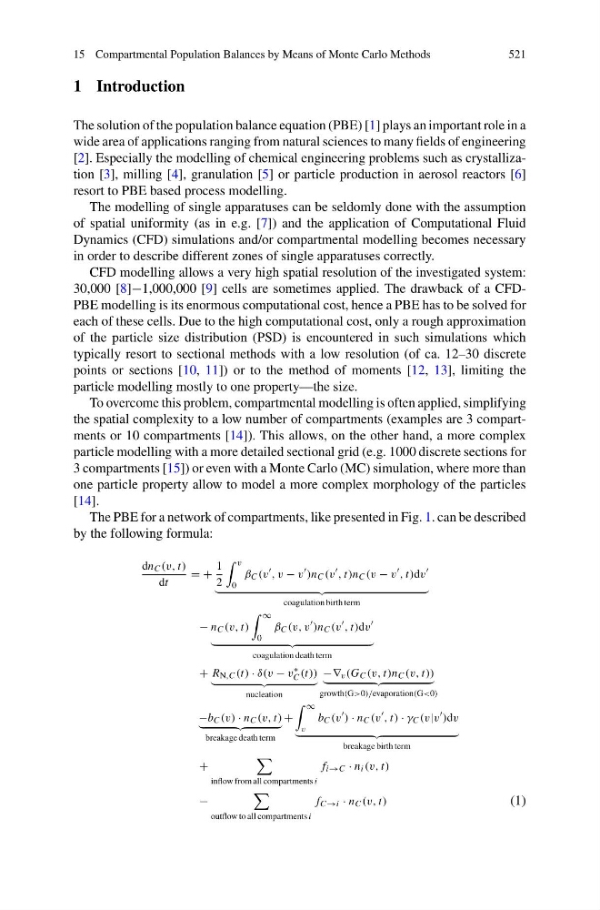
The PBE for a network of compartments, like presented in Fig. 1. can be described
by the following formula:
dn C (v, t)
dt
= +
1
2
v
0
β C (v
, v − v
)n C (v
, t)n C (v − v
, t)dv
coagulation birth term
− n C (v, t)
∞
0
β C (v, v
)n C (v
, t)dv
coagulation death term
+ R N,C (t) · δ(v − v
∗
C (t))
nucleation
−∇ v (G C (v, t)n C (v, t))
growth(G>0)/evaporation(G<0)
−b C (v) · n C (v, t)
breakage death term
+
∞
v
b C (v
) · n C (v
, t) · γ C (v|v
)dv
breakage birth term
+
inflow from all compartments i
f i→C · n i (v, t)
−
outflow to all compartments i
f C→i · n C (v, t)
(1)
521
1 Introduction
The solution of the population balance equation (PBE) [1] plays an important role in a
wide area of applications ranging from natural sciences to many fields of engineering
[2]. Especially the modelling of chemical engineering problems such as crystallization [3], milling [4], granulation [5] or particle production in aerosol reactors [6]
resort to PBE based process modelling.
The modelling of single apparatuses can be seldomly done with the assumption
of spatial uniformity (as in e.g. [7]) and the application of Computational Fluid
Dynamics (CFD) simulations and/or compartmental modelling becomes necessary
in order to describe different zones of single apparatuses correctly.
CFD modelling allows a very high spatial resolution of the investigated system:
30,000 [8]−1,000,000 [9] cells are sometimes applied. The drawback of a CFDPBE modelling is its enormous computational cost, hence a PBE has to be solved for
each of these cells. Due to the high computational cost, only a rough approximation
of the particle size distribution (PSD) is encountered in such simulations which
typically resort to sectional methods with a low resolution (of ca. 12–30 discrete
points or sections [10, 11]) or to the method of moments [12, 13], limiting the
particle modelling mostly to one property—the size.
To overcome this problem, compartmental modelling is often applied, simplifying
the spatial complexity to a low number of compartments (examples are 3 compartments or 10 compartments [14]). This allows, on the other hand, a more complex
particle modelling with a more detailed sectional grid (e.g. 1000 discrete sections for
3 compartments [15]) or even with a Monte Carlo (MC) simulation, where more than
one particle property allow to model a more complex morphology of the particles
[14].
The PBE for a network of compartments, like presented in Fig. 1. can be described
by the following formula:
dn C (v, t)
dt
= +
1
2
v
0
β C (v
, v − v
)n C (v
, t)n C (v − v
, t)dv
coagulation birth term
− n C (v, t)
∞
0
β C (v, v
)n C (v
, t)dv
coagulation death term
+ R N,C (t) · δ(v − v
∗
C (t))
nucleation
−∇ v (G C (v, t)n C (v, t))
growth(G>0)/evaporation(G<0)
−b C (v) · n C (v, t)
breakage death term
+
∞
v
b C (v
) · n C (v
, t) · γ C (v|v
)dv
breakage birth term
+
inflow from all compartments i
f i→C · n i (v, t)
−
outflow to all compartments i
f C→i · n C (v, t)
(1)