

14 Numerical Methods for Coupled Population Balance Systems …
509
n 1
2n 1
n 2
2n 2
n 3
2n 3
φ
F 1 (
φ)
F 2 (F 1 (
φ))
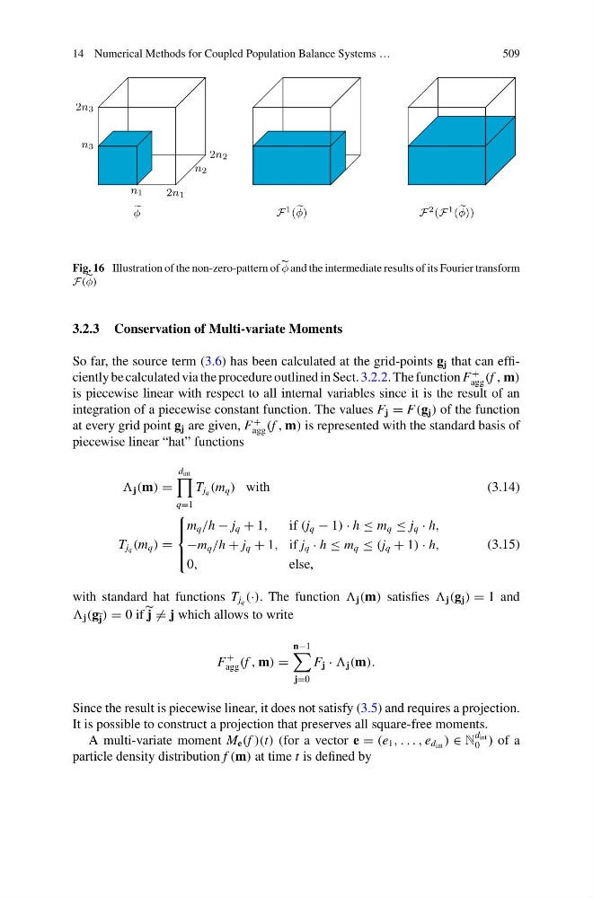
Fig. 16 Illustration of the non-zero-pattern of φ and the intermediate results of its Fourier transform
F ( φ)
3.2.3 Conservation of Multi-variate Moments
So far, the source term (3.6) has been calculated at the grid-points g j that can efficiently be calculated via the procedure outlined in Sect. 3.2.2. The function F
+
agg (f , m)
is piecewise linear with respect to all internal variables since it is the result of an
integration of a piecewise constant function. The values F j = F(g j ) of the function
at every grid point g j are given, F
+
agg (f , m) is represented with the standard basis of
piecewise linear “hat” functions
j (m) =
d int
q=1
T j q (m q ) with
(3.14)
T j q (m q ) =
⎧
⎪ ⎨
⎪ ⎩
m q /h − j q + 1,
if (j q − 1) · h ≤ m q ≤ j q · h,
−m q /h + j q + 1, if j q · h ≤ m q ≤ (j q + 1) · h,
0,
else,
(3.15)
with standard hat functions T j q (·). The function j (m) satisfies j (g j ) = 1 and
j (g j ) = 0 if j = j which allows to write
F
+
agg (f , m) =
n−1
j=0
F j · j (m).
Since the result is piecewise linear, it does not satisfy (3.5) and requires a projection.
It is possible to construct a projection that preserves all square-free moments.
A multi-variate moment M e (f )(t) (for a vector e = (e 1 , . . . , e d int ) ∈ N
d int
0 ) of a
particle density distribution f (m) at time t is defined by
509
n 1
2n 1
n 2
2n 2
n 3
2n 3
φ
F 1 (
φ)
F 2 (F 1 (
φ))
Fig. 16 Illustration of the non-zero-pattern of φ and the intermediate results of its Fourier transform
F ( φ)
3.2.3 Conservation of Multi-variate Moments
So far, the source term (3.6) has been calculated at the grid-points g j that can efficiently be calculated via the procedure outlined in Sect. 3.2.2. The function F
+
agg (f , m)
is piecewise linear with respect to all internal variables since it is the result of an
integration of a piecewise constant function. The values F j = F(g j ) of the function
at every grid point g j are given, F
+
agg (f , m) is represented with the standard basis of
piecewise linear “hat” functions
j (m) =
d int
q=1
T j q (m q ) with
(3.14)
T j q (m q ) =
⎧
⎪ ⎨
⎪ ⎩
m q /h − j q + 1,
if (j q − 1) · h ≤ m q ≤ j q · h,
−m q /h + j q + 1, if j q · h ≤ m q ≤ (j q + 1) · h,
0,
else,
(3.15)
with standard hat functions T j q (·). The function j (m) satisfies j (g j ) = 1 and
j (g j ) = 0 if j = j which allows to write
F
+
agg (f , m) =
n−1
j=0
F j · j (m).
Since the result is piecewise linear, it does not satisfy (3.5) and requires a projection.
It is possible to construct a projection that preserves all square-free moments.
A multi-variate moment M e (f )(t) (for a vector e = (e 1 , . . . , e d int ) ∈ N
d int
0 ) of a
particle density distribution f (m) at time t is defined by