

14 Numerical Methods for Coupled Population Balance Systems …
495
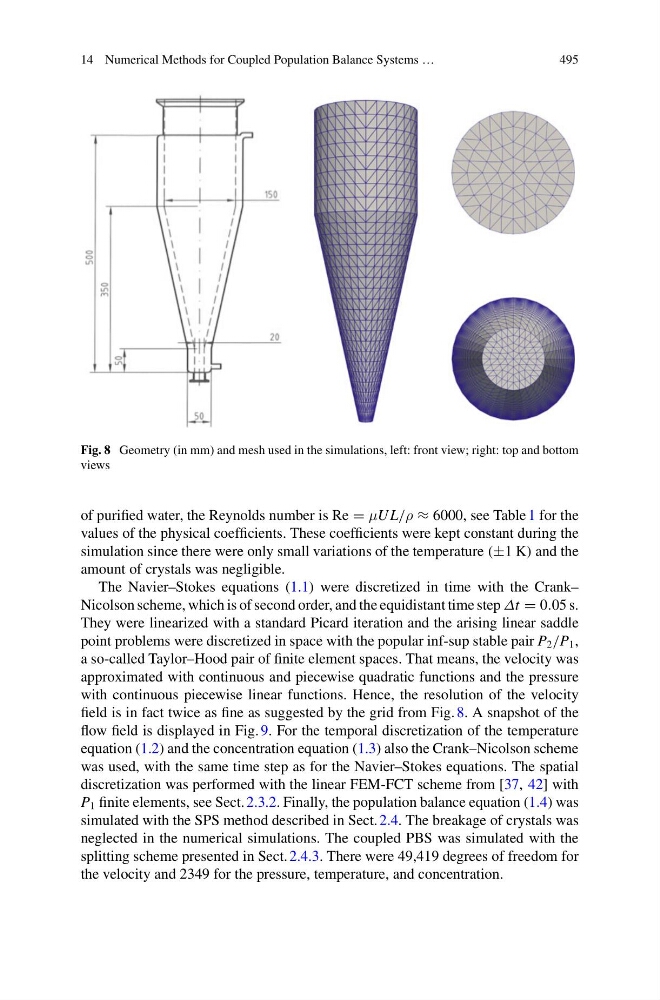
Fig. 8 Geometry (in mm) and mesh used in the simulations, left: front view; right: top and bottom
views
of purified water, the Reynolds number is Re = μU L/ρ ≈ 6000, see Table 1 for the
values of the physical coefficients. These coefficients were kept constant during the
simulation since there were only small variations of the temperature (±1 K) and the
amount of crystals was negligible.
The Navier–Stokes equations (1.1) were discretized in time with the Crank–
Nicolson scheme, which is of second order, and the equidistant time step Δt = 0.05 s.
They were linearized with a standard Picard iteration and the arising linear saddle
point problems were discretized in space with the popular inf-sup stable pair P 2 /P 1 ,
a so-called Taylor–Hood pair of finite element spaces. That means, the velocity was
approximated with continuous and piecewise quadratic functions and the pressure
with continuous piecewise linear functions. Hence, the resolution of the velocity
field is in fact twice as fine as suggested by the grid from Fig. 8. A snapshot of the
flow field is displayed in Fig. 9. For the temporal discretization of the temperature
equation (1.2) and the concentration equation (1.3) also the Crank–Nicolson scheme
was used, with the same time step as for the Navier–Stokes equations. The spatial
discretization was performed with the linear FEM-FCT scheme from [37, 42] with
P 1 finite elements, see Sect. 2.3.2. Finally, the population balance equation (1.4) was
simulated with the SPS method described in Sect. 2.4. The breakage of crystals was
neglected in the numerical simulations. The coupled PBS was simulated with the
splitting scheme presented in Sect. 2.4.3. There were 49,419 degrees of freedom for
the velocity and 2349 for the pressure, temperature, and concentration.
495
Fig. 8 Geometry (in mm) and mesh used in the simulations, left: front view; right: top and bottom
views
of purified water, the Reynolds number is Re = μU L/ρ ≈ 6000, see Table 1 for the
values of the physical coefficients. These coefficients were kept constant during the
simulation since there were only small variations of the temperature (±1 K) and the
amount of crystals was negligible.
The Navier–Stokes equations (1.1) were discretized in time with the Crank–
Nicolson scheme, which is of second order, and the equidistant time step Δt = 0.05 s.
They were linearized with a standard Picard iteration and the arising linear saddle
point problems were discretized in space with the popular inf-sup stable pair P 2 /P 1 ,
a so-called Taylor–Hood pair of finite element spaces. That means, the velocity was
approximated with continuous and piecewise quadratic functions and the pressure
with continuous piecewise linear functions. Hence, the resolution of the velocity
field is in fact twice as fine as suggested by the grid from Fig. 8. A snapshot of the
flow field is displayed in Fig. 9. For the temporal discretization of the temperature
equation (1.2) and the concentration equation (1.3) also the Crank–Nicolson scheme
was used, with the same time step as for the Navier–Stokes equations. The spatial
discretization was performed with the linear FEM-FCT scheme from [37, 42] with
P 1 finite elements, see Sect. 2.3.2. Finally, the population balance equation (1.4) was
simulated with the SPS method described in Sect. 2.4. The breakage of crystals was
neglected in the numerical simulations. The coupled PBS was simulated with the
splitting scheme presented in Sect. 2.4.3. There were 49,419 degrees of freedom for
the velocity and 2349 for the pressure, temperature, and concentration.