

278
M. Michaud et al.
J =
⎡
⎢
⎢
⎣
∂g 1
∂o 1
. . .
∂g 1
∂o m
. . .
. . .
. . .
∂g n
∂o 1
. . .
∂g n
∂o m
⎤
⎥
⎥
⎦ =
J R
J M
(16)
with:
J M =
∂g M
∂o
= M · exp o
J R =
ln(10)
2
· A ·
⎛
⎜
⎝
1
2
√
I
1 +
√
I
2 − b
⎞
⎟
⎠ · R · z
2
⊗
exp(o) ◦ z
2
+ R
(17)
For brevity, the following operators are used:
Matrix product: •
Hadamard product: °
Dyadic product: ⊗
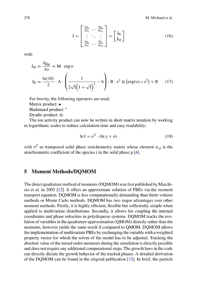
The ion activity product can now be written in short matrix notation by working
in logarithmic scales to reduce calculation time and easy readability:
ln I = σ
T
· (ln γ + o)
(18)
with σ
T as transposed solid phase stoichiometry matrix whose element σ i,p is the
stoichiometric coefficient of the species i in the solid phase p [4].
5 Moment Methods/DQMOM
The direct quadrature method of moments (DQMOM) was first published by Marchisio et al. in 2005 [12]. It offers an approximate solution of PBEs via the moment
transport equation. DQMOM is less computationally demanding than finite volume
methods or Monte Carlo methods. DQMOM has two major advantages over other
moment methods. Firstly, it is highly efficient, flexible but sufficiently simple when
applied to multivariate distributions. Secondly, it allows for coupling the internal
coordinates and phase velocities in polydisperse systems. DQMOM tracks the evolution of variables in the quadrature approximation (QMOM) directly rather than the
moments, however yields the same result if compared to QMOM. DQMOM allows
the implementation of multivariate PBEs by exchanging the variable with a weighted
property vector for which the solver of the model has to be adjusted. Tracking the
absolute value of the mixed order moments during the simulation is directly possible
and does not require any additional computational steps. The growth laws in the code
can directly dictate the growth behavior of the tracked phases. A detailed derivation
of the DQMOM can be found in the original publication [12]. In brief, the particle
M. Michaud et al.
J =
⎡
⎢
⎢
⎣
∂g 1
∂o 1
. . .
∂g 1
∂o m
. . .
. . .
. . .
∂g n
∂o 1
. . .
∂g n
∂o m
⎤
⎥
⎥
⎦ =
J R
J M
(16)
with:
J M =
∂g M
∂o
= M · exp o
J R =
ln(10)
2
· A ·
⎛
⎜
⎝
1
2
√
I
1 +
√
I
2 − b
⎞
⎟
⎠ · R · z
2
⊗
exp(o) ◦ z
2
+ R
(17)
For brevity, the following operators are used:
Matrix product: •
Hadamard product: °
Dyadic product: ⊗
The ion activity product can now be written in short matrix notation by working
in logarithmic scales to reduce calculation time and easy readability:
ln I = σ
T
· (ln γ + o)
(18)
with σ
T as transposed solid phase stoichiometry matrix whose element σ i,p is the
stoichiometric coefficient of the species i in the solid phase p [4].
5 Moment Methods/DQMOM
The direct quadrature method of moments (DQMOM) was first published by Marchisio et al. in 2005 [12]. It offers an approximate solution of PBEs via the moment
transport equation. DQMOM is less computationally demanding than finite volume
methods or Monte Carlo methods. DQMOM has two major advantages over other
moment methods. Firstly, it is highly efficient, flexible but sufficiently simple when
applied to multivariate distributions. Secondly, it allows for coupling the internal
coordinates and phase velocities in polydisperse systems. DQMOM tracks the evolution of variables in the quadrature approximation (QMOM) directly rather than the
moments, however yields the same result if compared to QMOM. DQMOM allows
the implementation of multivariate PBEs by exchanging the variable with a weighted
property vector for which the solver of the model has to be adjusted. Tracking the
absolute value of the mixed order moments during the simulation is directly possible
and does not require any additional computational steps. The growth laws in the code
can directly dictate the growth behavior of the tracked phases. A detailed derivation
of the DQMOM can be found in the original publication [12]. In brief, the particle