

5 Development of a Dynamic-Physical Process Model for Sieving
165
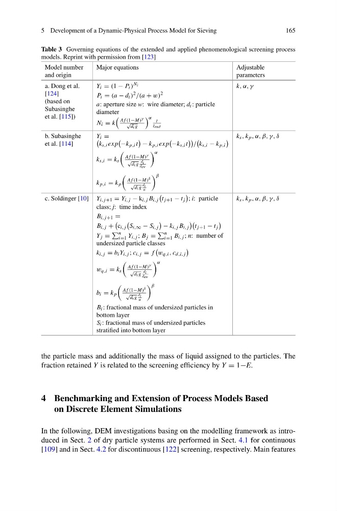
Table 3 Governing equations of the extended and applied phenomenological screening process
models. Reprint with permission from [123]
Model number
and origin
Major equations
Adjustable
parameters
a. Dong et al.
[124]
(based on
Subasinghe
et al. [115])
Y i = (1 − P i )
N i
P i = (a − d i )
2 /(a + w)
2
a: aperture size w: wire diameter; d i : particle
diameter
N i = k
A f (1−M) γ
√
d i g
α t
t end
k, α, γ
b. Subasinghe
et al. [114]
Y i =
k s,i ex p
−k p,i t
− k p,i ex p
−k s,i t
/
k s,i − k p,i
k s,i = k s
A f (1−M) γ
√
d i g
d i
dav
α
k p,i = k p
A f (1−M) δ
√
d i g
d i
a
β
k s , k p , α, β, γ, δ
c. Soldinger [10] Y i, j+1 = Y i, j − k i, j B i, j
t j+1 − t j
; i: particle
class; j: time index
B i, j+1 =
B i, j +
c i, j
S i,∞ − S i, j
− k i, j B i, j
t j+1 − t j
Y j =
n
i=1 Y i, j ; B j =
n
i=1 B i, j ; n: number of
undersized particle classes
k i, j = b i Y i, j ; c i, j = f
w q,i , c d,i, j
w q,i = k s
A f (1−M) γ
√
d i g
d i
dav
α
b i = k p
A f (1−M) δ
√
d i g
d i
a
β
B i : fractional mass of undersized particles in
bottom layer
S i : fractional mass of undersized particles
stratified into bottom layer
k s , k p , α, β, γ, δ
the particle mass and additionally the mass of liquid assigned to the particles. The
fraction retained Y is related to the screening efficiency by Y = 1−E.
4 Benchmarking and Extension of Process Models Based
on Discrete Element Simulations
In the following, DEM investigations basing on the modelling framework as introduced in Sect. 2 of dry particle systems are performed in Sect. 4.1 for continuous
[109] and in Sect. 4.2 for discontinuous [122] screening, respectively. Main features
165
Table 3 Governing equations of the extended and applied phenomenological screening process
models. Reprint with permission from [123]
Model number
and origin
Major equations
Adjustable
parameters
a. Dong et al.
[124]
(based on
Subasinghe
et al. [115])
Y i = (1 − P i )
N i
P i = (a − d i )
2 /(a + w)
2
a: aperture size w: wire diameter; d i : particle
diameter
N i = k
A f (1−M) γ
√
d i g
α t
t end
k, α, γ
b. Subasinghe
et al. [114]
Y i =
k s,i ex p
−k p,i t
− k p,i ex p
−k s,i t
/
k s,i − k p,i
k s,i = k s
A f (1−M) γ
√
d i g
d i
dav
α
k p,i = k p
A f (1−M) δ
√
d i g
d i
a
β
k s , k p , α, β, γ, δ
c. Soldinger [10] Y i, j+1 = Y i, j − k i, j B i, j
t j+1 − t j
; i: particle
class; j: time index
B i, j+1 =
B i, j +
c i, j
S i,∞ − S i, j
− k i, j B i, j
t j+1 − t j
Y j =
n
i=1 Y i, j ; B j =
n
i=1 B i, j ; n: number of
undersized particle classes
k i, j = b i Y i, j ; c i, j = f
w q,i , c d,i, j
w q,i = k s
A f (1−M) γ
√
d i g
d i
dav
α
b i = k p
A f (1−M) δ
√
d i g
d i
a
β
B i : fractional mass of undersized particles in
bottom layer
S i : fractional mass of undersized particles
stratified into bottom layer
k s , k p , α, β, γ, δ
the particle mass and additionally the mass of liquid assigned to the particles. The
fraction retained Y is related to the screening efficiency by Y = 1−E.
4 Benchmarking and Extension of Process Models Based
on Discrete Element Simulations
In the following, DEM investigations basing on the modelling framework as introduced in Sect. 2 of dry particle systems are performed in Sect. 4.1 for continuous
[109] and in Sect. 4.2 for discontinuous [122] screening, respectively. Main features