

154
D. Markauskas and H. Kruggel-Emden
a
b
c
d
e
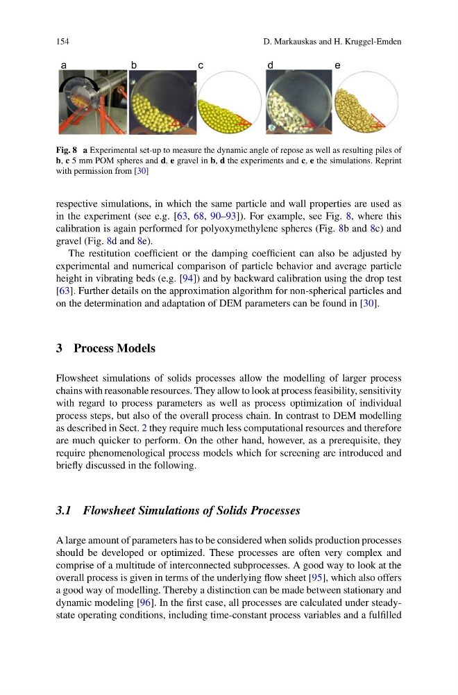
Fig. 8 a Experimental set-up to measure the dynamic angle of repose as well as resulting piles of
b, c 5 mm POM spheres and d, e gravel in b, d the experiments and c, e the simulations. Reprint
with permission from [30]
respective simulations, in which the same particle and wall properties are used as
in the experiment (see e.g. [63, 68, 90–93]). For example, see Fig. 8, where this
calibration is again performed for polyoxymethylene spheres (Fig. 8b and 8c) and
gravel (Fig. 8d and 8e).
The restitution coefficient or the damping coefficient can also be adjusted by
experimental and numerical comparison of particle behavior and average particle
height in vibrating beds (e.g. [94]) and by backward calibration using the drop test
[63]. Further details on the approximation algorithm for non-spherical particles and
on the determination and adaptation of DEM parameters can be found in [30].
3 Process Models
Flowsheet simulations of solids processes allow the modelling of larger process
chains with reasonable resources. They allow to look at process feasibility, sensitivity
with regard to process parameters as well as process optimization of individual
process steps, but also of the overall process chain. In contrast to DEM modelling
as described in Sect. 2 they require much less computational resources and therefore
are much quicker to perform. On the other hand, however, as a prerequisite, they
require phenomenological process models which for screening are introduced and
briefly discussed in the following.
3.1 Flowsheet Simulations of Solids Processes
A large amount of parameters has to be considered when solids production processes
should be developed or optimized. These processes are often very complex and
comprise of a multitude of interconnected subprocesses. A good way to look at the
overall process is given in terms of the underlying flow sheet [95], which also offers
a good way of modelling. Thereby a distinction can be made between stationary and
dynamic modeling [96]. In the first case, all processes are calculated under steadystate operating conditions, including time-constant process variables and a fulfilled
D. Markauskas and H. Kruggel-Emden
a
b
c
d
e
Fig. 8 a Experimental set-up to measure the dynamic angle of repose as well as resulting piles of
b, c 5 mm POM spheres and d, e gravel in b, d the experiments and c, e the simulations. Reprint
with permission from [30]
respective simulations, in which the same particle and wall properties are used as
in the experiment (see e.g. [63, 68, 90–93]). For example, see Fig. 8, where this
calibration is again performed for polyoxymethylene spheres (Fig. 8b and 8c) and
gravel (Fig. 8d and 8e).
The restitution coefficient or the damping coefficient can also be adjusted by
experimental and numerical comparison of particle behavior and average particle
height in vibrating beds (e.g. [94]) and by backward calibration using the drop test
[63]. Further details on the approximation algorithm for non-spherical particles and
on the determination and adaptation of DEM parameters can be found in [30].
3 Process Models
Flowsheet simulations of solids processes allow the modelling of larger process
chains with reasonable resources. They allow to look at process feasibility, sensitivity
with regard to process parameters as well as process optimization of individual
process steps, but also of the overall process chain. In contrast to DEM modelling
as described in Sect. 2 they require much less computational resources and therefore
are much quicker to perform. On the other hand, however, as a prerequisite, they
require phenomenological process models which for screening are introduced and
briefly discussed in the following.
3.1 Flowsheet Simulations of Solids Processes
A large amount of parameters has to be considered when solids production processes
should be developed or optimized. These processes are often very complex and
comprise of a multitude of interconnected subprocesses. A good way to look at the
overall process is given in terms of the underlying flow sheet [95], which also offers
a good way of modelling. Thereby a distinction can be made between stationary and
dynamic modeling [96]. In the first case, all processes are calculated under steadystate operating conditions, including time-constant process variables and a fulfilled