

150
D. Markauskas and H. Kruggel-Emden
ϕ iw =
2S/r i
1 + V lb /
πr i S 2
.
(15)
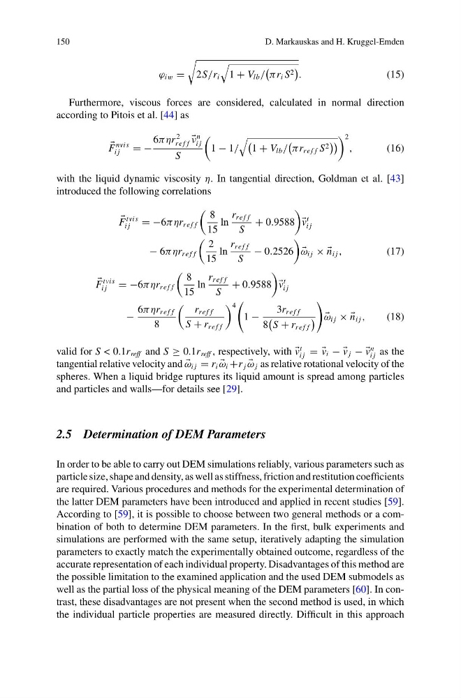
Furthermore, viscous forces are considered, calculated in normal direction
according to Pitois et al. [44] as
F
nvis
i j
= −
6πηr
2
re f f
ν
n
i j
S
1 − 1/
1 + V lb /
πr re f f S 2
2
,
(16)
with the liquid dynamic viscosity η. In tangential direction, Goldman et al. [43]
introduced the following correlations
F
tvis
i j
= −6πηr re f f
8
15
ln
r re f f
S
+ 0.9588
v
t
i j
− 6πηr re f f
2
15
ln
r re f f
S
− 0.2526
ω i j × ×
n i j ,
(17)
F
tvis
i j
= −6πηr re f f
8
15
ln
r re f f
S
+ 0.9588
v
t
i j
−
6πηr re f f
8
r re f f
S + r re f f
4
1 −
3r re f f
8
S + r re f f
ω i j × ×
n i j ,
(18)
valid for S < 0.1r reff and S ≥ 0.1r reff , respectively, with
v
t
i j = =
v i − −
v j − −
v
n
i j as the
tangential relative velocity and
ω i j = r i
ω i +r j
ω j as relative rotational velocity of the
spheres. When a liquid bridge ruptures its liquid amount is spread among particles
and particles and walls—for details see [29].
2.5 Determination of DEM Parameters
In order to be able to carry out DEM simulations reliably, various parameters such as
particle size, shape and density, as well as stiffness, friction and restitution coefficients
are required. Various procedures and methods for the experimental determination of
the latter DEM parameters have been introduced and applied in recent studies [59].
According to [59], it is possible to choose between two general methods or a combination of both to determine DEM parameters. In the first, bulk experiments and
simulations are performed with the same setup, iteratively adapting the simulation
parameters to exactly match the experimentally obtained outcome, regardless of the
accurate representation of each individual property. Disadvantages of this method are
the possible limitation to the examined application and the used DEM submodels as
well as the partial loss of the physical meaning of the DEM parameters [60]. In contrast, these disadvantages are not present when the second method is used, in which
the individual particle properties are measured directly. Difficult in this approach
D. Markauskas and H. Kruggel-Emden
ϕ iw =
2S/r i
1 + V lb /
πr i S 2
.
(15)
Furthermore, viscous forces are considered, calculated in normal direction
according to Pitois et al. [44] as
F
nvis
i j
= −
6πηr
2
re f f
ν
n
i j
S
1 − 1/
1 + V lb /
πr re f f S 2
2
,
(16)
with the liquid dynamic viscosity η. In tangential direction, Goldman et al. [43]
introduced the following correlations
F
tvis
i j
= −6πηr re f f
8
15
ln
r re f f
S
+ 0.9588
v
t
i j
− 6πηr re f f
2
15
ln
r re f f
S
− 0.2526
ω i j × ×
n i j ,
(17)
F
tvis
i j
= −6πηr re f f
8
15
ln
r re f f
S
+ 0.9588
v
t
i j
−
6πηr re f f
8
r re f f
S + r re f f
4
1 −
3r re f f
8
S + r re f f
ω i j × ×
n i j ,
(18)
valid for S < 0.1r reff and S ≥ 0.1r reff , respectively, with
v
t
i j = =
v i − −
v j − −
v
n
i j as the
tangential relative velocity and
ω i j = r i
ω i +r j
ω j as relative rotational velocity of the
spheres. When a liquid bridge ruptures its liquid amount is spread among particles
and particles and walls—for details see [29].
2.5 Determination of DEM Parameters
In order to be able to carry out DEM simulations reliably, various parameters such as
particle size, shape and density, as well as stiffness, friction and restitution coefficients
are required. Various procedures and methods for the experimental determination of
the latter DEM parameters have been introduced and applied in recent studies [59].
According to [59], it is possible to choose between two general methods or a combination of both to determine DEM parameters. In the first, bulk experiments and
simulations are performed with the same setup, iteratively adapting the simulation
parameters to exactly match the experimentally obtained outcome, regardless of the
accurate representation of each individual property. Disadvantages of this method are
the possible limitation to the examined application and the used DEM submodels as
well as the partial loss of the physical meaning of the DEM parameters [60]. In contrast, these disadvantages are not present when the second method is used, in which
the individual particle properties are measured directly. Difficult in this approach