

4 Dynamic Simulation of Technical Precipitation Processes
127
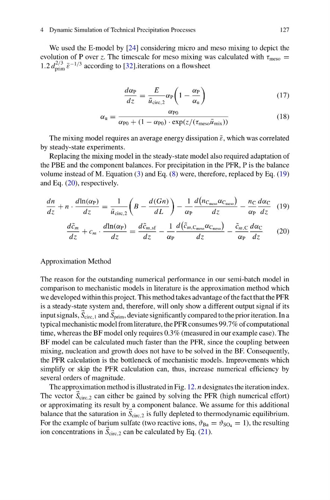
We used the E-model by [24] considering micro and meso mixing to depict the
evolution of P over z. The timescale for meso mixing was calculated with τ meso =
1.2 d
2/3
prim ¯
ε
−1/3 according to [32].iterations on a flowsheet
dα P
dz
=
E
¯
u circ,2
α P
1 −
α P
α u
(17)
α u =
α P0
α P0 + (1 − α P0 ) · exp(z/(τ meso ¯
u mix ))
(18)
The mixing model requires an average energy dissipation ¯
ε, which was correlated
by steady-state experiments.
Replacing the mixing model in the steady-state model also required adaptation of
the PBE and the component balances. For precipitation in the PFR, P is the balance
volume instead of M. Equation (3) and Eq. (8) were, therefore, replaced by Eq. (19)
and Eq. (20), respectively.
dn
dz
+ n ·
dln(α P )
dz
=
1
¯
u circ,2
B −
d(Gn)
d L
−
1
α P
d
n C meso α C meso
dz
−
n C
α P
dα C
dz
(19)
d ˜
c m
dz
+ c m ·
dln(α P )
dz
=
d ˜
c m,sf
dz
−
1
α P
d
˜
c m,C meso α C meso
dz
−
˜
c m,C
α P
dα C
dz
(20)
Approximation Method
The reason for the outstanding numerical performance in our semi-batch model in
comparison to mechanistic models in literature is the approximation method which
we developed within this project. This method takes advantage of the fact that the PFR
is a steady-state system and, therefore, will only show a different output signal if its
input signals,
S circ,1 and
S prim , deviate significantly compared to the prior iteration. In a
typical mechanistic model from literature, the PFR consumes 99.7% of computational
time, whereas the BF model only requires 0.3% (measured in our example case). The
BF model can be calculated much faster than the PFR, since the coupling between
mixing, nucleation and growth does not have to be solved in the BF. Consequently,
the PFR calculation is the bottleneck of mechanistic models. Improvements which
simplify or skip the PFR calculation can, thus, increase numerical efficiency by
several orders of magnitude.
The approximation method is illustrated in Fig. 12. n designates the iteration index.
The vector
S circ,2 can either be gained by solving the PFR (high numerical effort)
or approximating its result by a component balance. We assume for this additional
balance that the saturation in
S circ,2 is fully depleted to thermodynamic equilibrium.
For the example of barium sulfate (two reactive ions, ϑ Ba = ϑ SO 4 = 1), the resulting
ion concentrations in
S circ,2 can be calculated by Eq. (21).
127
We used the E-model by [24] considering micro and meso mixing to depict the
evolution of P over z. The timescale for meso mixing was calculated with τ meso =
1.2 d
2/3
prim ¯
ε
−1/3 according to [32].iterations on a flowsheet
dα P
dz
=
E
¯
u circ,2
α P
1 −
α P
α u
(17)
α u =
α P0
α P0 + (1 − α P0 ) · exp(z/(τ meso ¯
u mix ))
(18)
The mixing model requires an average energy dissipation ¯
ε, which was correlated
by steady-state experiments.
Replacing the mixing model in the steady-state model also required adaptation of
the PBE and the component balances. For precipitation in the PFR, P is the balance
volume instead of M. Equation (3) and Eq. (8) were, therefore, replaced by Eq. (19)
and Eq. (20), respectively.
dn
dz
+ n ·
dln(α P )
dz
=
1
¯
u circ,2
B −
d(Gn)
d L
−
1
α P
d
n C meso α C meso
dz
−
n C
α P
dα C
dz
(19)
d ˜
c m
dz
+ c m ·
dln(α P )
dz
=
d ˜
c m,sf
dz
−
1
α P
d
˜
c m,C meso α C meso
dz
−
˜
c m,C
α P
dα C
dz
(20)
Approximation Method
The reason for the outstanding numerical performance in our semi-batch model in
comparison to mechanistic models in literature is the approximation method which
we developed within this project. This method takes advantage of the fact that the PFR
is a steady-state system and, therefore, will only show a different output signal if its
input signals,
S circ,1 and
S prim , deviate significantly compared to the prior iteration. In a
typical mechanistic model from literature, the PFR consumes 99.7% of computational
time, whereas the BF model only requires 0.3% (measured in our example case). The
BF model can be calculated much faster than the PFR, since the coupling between
mixing, nucleation and growth does not have to be solved in the BF. Consequently,
the PFR calculation is the bottleneck of mechanistic models. Improvements which
simplify or skip the PFR calculation can, thus, increase numerical efficiency by
several orders of magnitude.
The approximation method is illustrated in Fig. 12. n designates the iteration index.
The vector
S circ,2 can either be gained by solving the PFR (high numerical effort)
or approximating its result by a component balance. We assume for this additional
balance that the saturation in
S circ,2 is fully depleted to thermodynamic equilibrium.
For the example of barium sulfate (two reactive ions, ϑ Ba = ϑ SO 4 = 1), the resulting
ion concentrations in
S circ,2 can be calculated by Eq. (21).