

3.2 Response of Damped Systems to Harmonic Loading
63
The maximum value of the dynamic load factor is known as the magnification factor (μ), i.e. the ratio of the maximum dynamic displacement to the static
displacement is defined as the magnification factor and is given by
μ =
1
1 − η 2
2 + ( 2ηζ ) 2
(3.18)
The magnification factor is of interest to the designer. A magnification factor of
3 immediately reveals that all maximum displacements, forces and stresses due to
dynamic load will be thrice the value obtained from the static analysis.
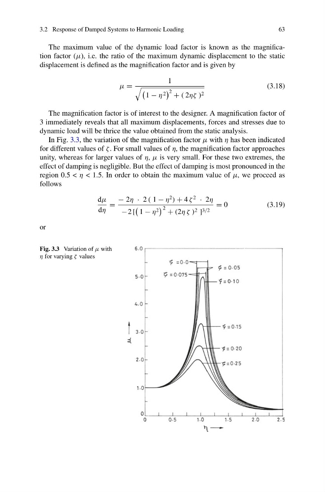
In Fig. 3.3, the variation of the magnification factor μ with η has been indicated
for different values of ζ. For small values of η, the magnification factor approaches
unity, whereas for larger values of η, μ is very small. For these two extremes, the
effect of damping is negligible. But the effect of damping is most pronounced in the
region 0.5 < η < 1.5. In order to obtain the maximum value of μ, we proceed as
follows
dμ
dη
=
− 2η · 2 ( 1 − η
2
) + 4 ζ
2
· 2η
−2 [
1 − η 2
2 + (2η ζ ) 2 ] 3/2
= 0
(3.19)
or
Fig. 3.3 Variation of μ with
η for varying ζ values
63
The maximum value of the dynamic load factor is known as the magnification factor (μ), i.e. the ratio of the maximum dynamic displacement to the static
displacement is defined as the magnification factor and is given by
μ =
1
1 − η 2
2 + ( 2ηζ ) 2
(3.18)
The magnification factor is of interest to the designer. A magnification factor of
3 immediately reveals that all maximum displacements, forces and stresses due to
dynamic load will be thrice the value obtained from the static analysis.
In Fig. 3.3, the variation of the magnification factor μ with η has been indicated
for different values of ζ. For small values of η, the magnification factor approaches
unity, whereas for larger values of η, μ is very small. For these two extremes, the
effect of damping is negligible. But the effect of damping is most pronounced in the
region 0.5 < η < 1.5. In order to obtain the maximum value of μ, we proceed as
follows
dμ
dη
=
− 2η · 2 ( 1 − η
2
) + 4 ζ
2
· 2η
−2 [
1 − η 2
2 + (2η ζ ) 2 ] 3/2
= 0
(3.19)
or
Fig. 3.3 Variation of μ with
η for varying ζ values