

538
15 Random Vibrations
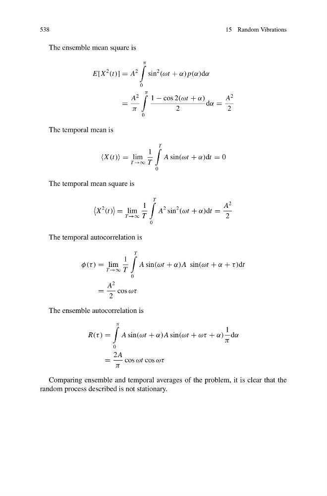
The ensemble mean square is
E[X
2
(t)] = A
2
π
0
sin
2
(ωt + α) p(α)dα
=
A
2
π
π
0
1 − cos 2(ωt + α)
2
dα =
A
2
2
The temporal mean is
X (t) = lim
T →∞
1
T
T
0
A sin(ωt + α)dt = 0
The temporal mean square is
X
2
(t)
= lim
T →∞
1
T
T
0
A
2 sin
2
(ωt + α)dt =
A
2
2
The temporal autocorrelation is
φ(τ ) = lim
T →∞
1
T
T
0
A sin(ωt + α)A sin(ωt + α + τ )dt
=
A
2
2
cos ωτ
The ensemble autocorrelation is
R(τ ) =
π
0
A sin(ωt + α)A sin(ωt + ωτ + α)
1
π
dα
=
2 A
π
cos ωt cos ωτ
Comparing ensemble and temporal averages of the problem, it is clear that the
random process described is not stationary.
15 Random Vibrations
The ensemble mean square is
E[X
2
(t)] = A
2
π
0
sin
2
(ωt + α) p(α)dα
=
A
2
π
π
0
1 − cos 2(ωt + α)
2
dα =
A
2
2
The temporal mean is
X (t) = lim
T →∞
1
T
T
0
A sin(ωt + α)dt = 0
The temporal mean square is
X
2
(t)
= lim
T →∞
1
T
T
0
A
2 sin
2
(ωt + α)dt =
A
2
2
The temporal autocorrelation is
φ(τ ) = lim
T →∞
1
T
T
0
A sin(ωt + α)A sin(ωt + α + τ )dt
=
A
2
2
cos ωτ
The ensemble autocorrelation is
R(τ ) =
π
0
A sin(ωt + α)A sin(ωt + ωτ + α)
1
π
dα
=
2 A
π
cos ωt cos ωτ
Comparing ensemble and temporal averages of the problem, it is clear that the
random process described is not stationary.