

494
13 Finite Difference Method for the Vibration Analysis …
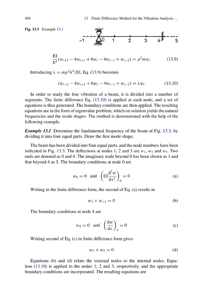
Fig. 13.3 Example 13.1
EI
h 4 (w i+2 − 4w i+1 + 6w i − 4w i−1 + w i−2 ) = p
2 mw i
(13.9)
Introducing λ = mp
2 h
4
/EI, Eq. (13.9) becomes
(w i+2 − 4w i+1 + 6w i − 4w i−1 + w i−2 ) = λw i
(13.10)
In order to study the free vibration of a beam, it is divided into a number of
segments. The finite difference Eq. (13.10) is applied at each node, and a set of
equations is thus generated. The boundary conditions are then applied. The resulting
equations are in the form of eigenvalue problem, which on solution yields the natural
frequencies and the mode shapes. The method is demonstrated with the help of the
following example.
Example 13.1 Determine the fundamental frequency of the beam of Fig. 13.3, by
dividing it into four equal parts. Draw the first mode shape.
The beam has been divided into four equal parts, and the node numbers have been
indicated in Fig. 13.3. The deflections at nodes 1, 2 and 3 are w 1 , w 2 and w 3 . Two
ends are denoted as 0 and 4. The imaginary node beyond 0 has been shown as 1 and
that beyond 4 as 5. The boundary conditions at node 0 are
w 0 = 0 and
EI
d
2
w
dx 2
0
= 0
( a )
Writing in the finite difference form, the second of Eq. (a) results in
w 1 + w −1 = 0
( b )
The boundary conditions at node 4 are
w 4 = 0 and
dw
dx
4
= 0
( c )
Writing second of Eq. (c) in finite difference form gives
w 3 + w 5 = 0
( d )
Equations (b) and (d) relate the external nodes to the internal nodes. Equation (13.10) is applied to the nodes 1, 2 and 3, respectively, and the appropriate
boundary conditions are incorporated. The resulting equations are
13 Finite Difference Method for the Vibration Analysis …
Fig. 13.3 Example 13.1
EI
h 4 (w i+2 − 4w i+1 + 6w i − 4w i−1 + w i−2 ) = p
2 mw i
(13.9)
Introducing λ = mp
2 h
4
/EI, Eq. (13.9) becomes
(w i+2 − 4w i+1 + 6w i − 4w i−1 + w i−2 ) = λw i
(13.10)
In order to study the free vibration of a beam, it is divided into a number of
segments. The finite difference Eq. (13.10) is applied at each node, and a set of
equations is thus generated. The boundary conditions are then applied. The resulting
equations are in the form of eigenvalue problem, which on solution yields the natural
frequencies and the mode shapes. The method is demonstrated with the help of the
following example.
Example 13.1 Determine the fundamental frequency of the beam of Fig. 13.3, by
dividing it into four equal parts. Draw the first mode shape.
The beam has been divided into four equal parts, and the node numbers have been
indicated in Fig. 13.3. The deflections at nodes 1, 2 and 3 are w 1 , w 2 and w 3 . Two
ends are denoted as 0 and 4. The imaginary node beyond 0 has been shown as 1 and
that beyond 4 as 5. The boundary conditions at node 0 are
w 0 = 0 and
EI
d
2
w
dx 2
0
= 0
( a )
Writing in the finite difference form, the second of Eq. (a) results in
w 1 + w −1 = 0
( b )
The boundary conditions at node 4 are
w 4 = 0 and
dw
dx
4
= 0
( c )
Writing second of Eq. (c) in finite difference form gives
w 3 + w 5 = 0
( d )
Equations (b) and (d) relate the external nodes to the internal nodes. Equation (13.10) is applied to the nodes 1, 2 and 3, respectively, and the appropriate
boundary conditions are incorporated. The resulting equations are