

12.9 Periodic Structures
483
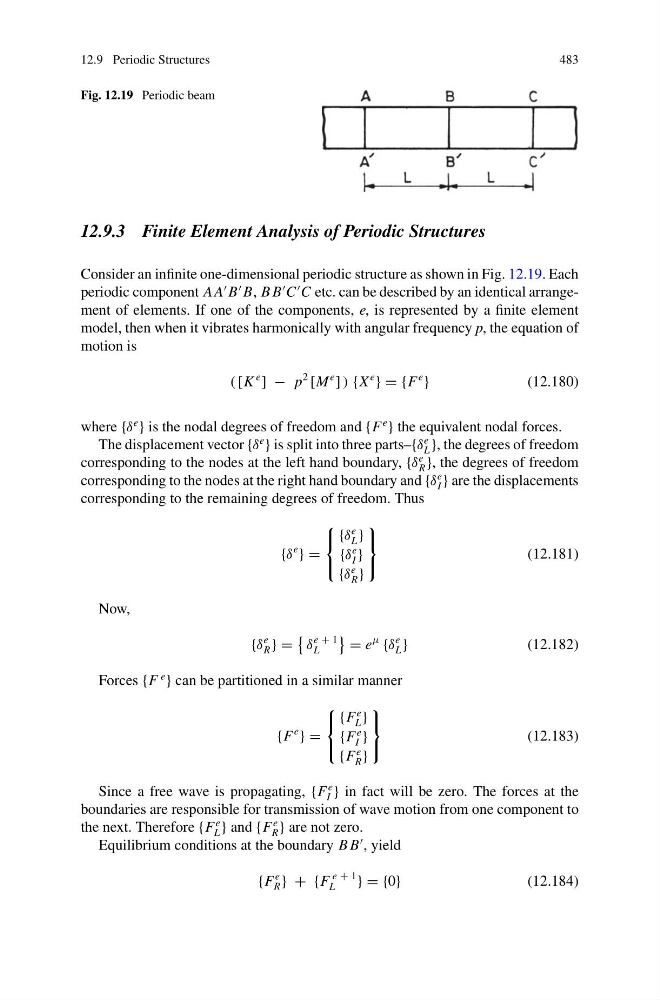
Fig. 12.19 Periodic beam
12.9.3 Finite Element Analysis of Periodic Structures
Consider an infinite one-dimensional periodic structure as shown in Fig. 12.19. Each
periodic component A A
B
B, B B
C
C etc. can be described by an identical arrangement of elements. If one of the components, e, is represented by a finite element
model, then when it vibrates harmonically with angular frequency p, the equation of
motion is
( [K
e
] − p
2
[M
e
] ) {X
e
} = {F
e
}
(12.180)
where {δ
e
} is the nodal degrees of freedom and {F
e
} the equivalent nodal forces.
The displacement vector {δ
e
} is split into three parts–{δ
e
L }, the degrees of freedom
corresponding to the nodes at the left hand boundary, {δ
e
R }, the degrees of freedom
corresponding to the nodes at the right hand boundary and {δ
e
I } are the displacements
corresponding to the remaining degrees of freedom. Thus
{δ
e
} =
⎧
⎨
⎩
{δ
e
L }
{δ
e
I }
{δ
e
R }
⎫
⎬
⎭
(12.181)
Now,
{δ
e
R } =
δ
e + 1
L
= e
μ
{δ
e
L }
(12.182)
Forces {F
e
} can be partitioned in a similar manner
{F
e
} =
⎧
⎨
⎩
{F
e
L }
{F
e
I }
{F
e
R }
⎫
⎬
⎭
(12.183)
Since a free wave is propagating, {F
e
I } in fact will be zero. The forces at the
boundaries are responsible for transmission of wave motion from one component to
the next. Therefore {F
e
L } and {F
e
R } are not zero.
Equilibrium conditions at the boundary B B
, yield
{F
e
R } + {F
e + 1
L
} = {0}
(12.184)
483
Fig. 12.19 Periodic beam
12.9.3 Finite Element Analysis of Periodic Structures
Consider an infinite one-dimensional periodic structure as shown in Fig. 12.19. Each
periodic component A A
B
B, B B
C
C etc. can be described by an identical arrangement of elements. If one of the components, e, is represented by a finite element
model, then when it vibrates harmonically with angular frequency p, the equation of
motion is
( [K
e
] − p
2
[M
e
] ) {X
e
} = {F
e
}
(12.180)
where {δ
e
} is the nodal degrees of freedom and {F
e
} the equivalent nodal forces.
The displacement vector {δ
e
} is split into three parts–{δ
e
L }, the degrees of freedom
corresponding to the nodes at the left hand boundary, {δ
e
R }, the degrees of freedom
corresponding to the nodes at the right hand boundary and {δ
e
I } are the displacements
corresponding to the remaining degrees of freedom. Thus
{δ
e
} =
⎧
⎨
⎩
{δ
e
L }
{δ
e
I }
{δ
e
R }
⎫
⎬
⎭
(12.181)
Now,
{δ
e
R } =
δ
e + 1
L
= e
μ
{δ
e
L }
(12.182)
Forces {F
e
} can be partitioned in a similar manner
{F
e
} =
⎧
⎨
⎩
{F
e
L }
{F
e
I }
{F
e
R }
⎫
⎬
⎭
(12.183)
Since a free wave is propagating, {F
e
I } in fact will be zero. The forces at the
boundaries are responsible for transmission of wave motion from one component to
the next. Therefore {F
e
L } and {F
e
R } are not zero.
Equilibrium conditions at the boundary B B
, yield
{F
e
R } + {F
e + 1
L
} = {0}
(12.184)