

454
12 Finite Element Method in Vibration Analysis
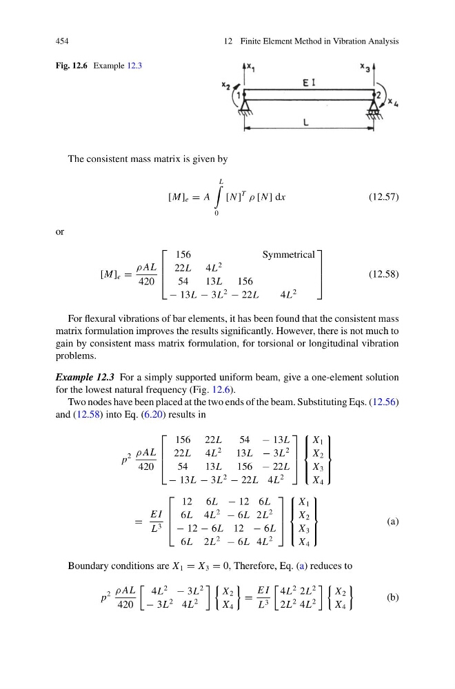
Fig. 12.6 Example 12.3
The consistent mass matrix is given by
[M] e = A
L
0
[N ]
T
ρ [N ] dx
(12.57)
or
[M] e =
ρ AL
420
⎡
⎢
⎢
⎣
156
Symmetrical
22L 4L
2
54
13L 156
− 13L − 3L
2
− 22L
4L
2
⎤
⎥
⎥
⎦
(12.58)
For flexural vibrations of bar elements, it has been found that the consistent mass
matrix formulation improves the results significantly. However, there is not much to
gain by consistent mass matrix formulation, for torsional or longitudinal vibration
problems.
Example 12.3 For a simply supported uniform beam, give a one-element solution
for the lowest natural frequency (Fig. 12.6).
Two nodes have been placed at the two ends of the beam. Substituting Eqs. (12.56)
and (12.58) into Eq. (6.20) results in
p
2 ρ AL
420
⎡
⎢
⎢
⎣
156 22L
54 − 13L
22L 4L
2
13L − 3L
2
54
13L 156 − 22L
− 13L − 3L
2
− 22L 4L
2
⎤
⎥
⎥
⎦
⎧
⎪ ⎪ ⎨
⎪ ⎪ ⎩
X 1
X 2
X 3
X 4
⎫
⎪ ⎪ ⎬
⎪ ⎪ ⎭
=
E I
L 3
⎡
⎢
⎢
⎣
12 6L − 12 6L
6L 4L
2
− 6L 2L
2
− 12 − 6L 12 − 6L
6L 2L
2
− 6L 4L
2
⎤
⎥
⎥
⎦
⎧
⎪ ⎪ ⎨
⎪ ⎪ ⎩
X 1
X 2
X 3
X 4
⎫
⎪ ⎪ ⎬
⎪ ⎪ ⎭
(a)
Boundary conditions are X 1 = X 3 = 0, Therefore, Eq. (a) reduces to
p
2 ρ AL
420
4L
2
− 3L
2
− 3L
2 4L
2
X 2
X 4
=
E I
L 3
4L
2 2L
2
2L
2 4L
2
X 2
X 4
(b)
12 Finite Element Method in Vibration Analysis
Fig. 12.6 Example 12.3
The consistent mass matrix is given by
[M] e = A
L
0
[N ]
T
ρ [N ] dx
(12.57)
or
[M] e =
ρ AL
420
⎡
⎢
⎢
⎣
156
Symmetrical
22L 4L
2
54
13L 156
− 13L − 3L
2
− 22L
4L
2
⎤
⎥
⎥
⎦
(12.58)
For flexural vibrations of bar elements, it has been found that the consistent mass
matrix formulation improves the results significantly. However, there is not much to
gain by consistent mass matrix formulation, for torsional or longitudinal vibration
problems.
Example 12.3 For a simply supported uniform beam, give a one-element solution
for the lowest natural frequency (Fig. 12.6).
Two nodes have been placed at the two ends of the beam. Substituting Eqs. (12.56)
and (12.58) into Eq. (6.20) results in
p
2 ρ AL
420
⎡
⎢
⎢
⎣
156 22L
54 − 13L
22L 4L
2
13L − 3L
2
54
13L 156 − 22L
− 13L − 3L
2
− 22L 4L
2
⎤
⎥
⎥
⎦
⎧
⎪ ⎪ ⎨
⎪ ⎪ ⎩
X 1
X 2
X 3
X 4
⎫
⎪ ⎪ ⎬
⎪ ⎪ ⎭
=
E I
L 3
⎡
⎢
⎢
⎣
12 6L − 12 6L
6L 4L
2
− 6L 2L
2
− 12 − 6L 12 − 6L
6L 2L
2
− 6L 4L
2
⎤
⎥
⎥
⎦
⎧
⎪ ⎪ ⎨
⎪ ⎪ ⎩
X 1
X 2
X 3
X 4
⎫
⎪ ⎪ ⎬
⎪ ⎪ ⎭
(a)
Boundary conditions are X 1 = X 3 = 0, Therefore, Eq. (a) reduces to
p
2 ρ AL
420
4L
2
− 3L
2
− 3L
2 4L
2
X 2
X 4
=
E I
L 3
4L
2 2L
2
2L
2 4L
2
X 2
X 4
(b)