

452
12 Finite Element Method in Vibration Analysis
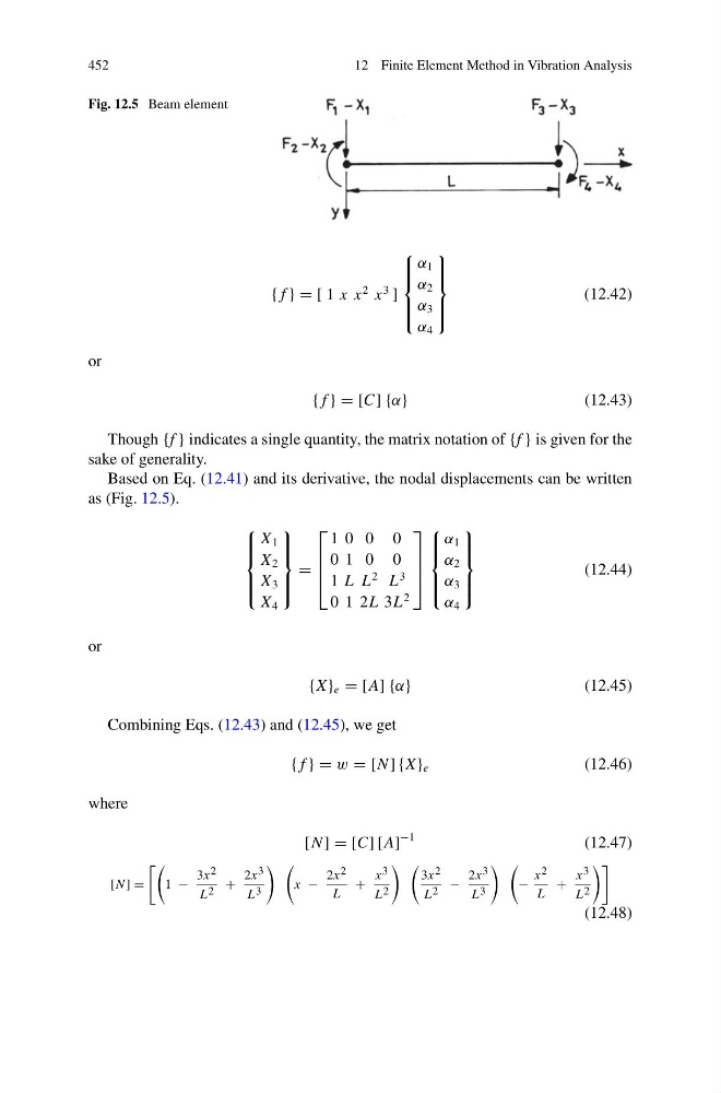
Fig. 12.5 Beam element
{ f } = [ 1 x x
2 x
3 ]
⎧
⎪ ⎪ ⎨
⎪ ⎪ ⎩
α 1
α 2
α 3
α 4
⎫
⎪ ⎪ ⎬
⎪ ⎪ ⎭
(12.42)
or
{ f } = [C] {α}
(12.43)
Though {f } indicates a single quantity, the matrix notation of {f } is given for the
sake of generality.
Based on Eq. (12.41) and its derivative, the nodal displacements can be written
as (Fig. 12.5).
⎧
⎪ ⎪ ⎨
⎪ ⎪ ⎩
X 1
X 2
X 3
X 4
⎫
⎪ ⎪ ⎬
⎪ ⎪ ⎭
=
⎡
⎢
⎢
⎣
1 0 0 0
0 1 0 0
1 L L
2 L
3
0 1 2L 3L
2
⎤
⎥
⎥
⎦
⎧
⎪ ⎪ ⎨
⎪ ⎪ ⎩
α 1
α 2
α 3
α 4
⎫
⎪ ⎪ ⎬
⎪ ⎪ ⎭
(12.44)
or
{X } e = [A] {α}
(12.45)
Combining Eqs. (12.43) and (12.45), we get
{ f } = w = [N ] {X } e
(12.46)
where
[N ] = [C] [A]
−1
(12.47)
[N ] =
1 −
3x 2
L 2 +
2x 3
L 3
x −
2x 2
L
+
x 3
L 2
3x 2
L 2 −
2x 3
L 3
−
x 2
L
+
x 3
L 2
(12.48)
12 Finite Element Method in Vibration Analysis
Fig. 12.5 Beam element
{ f } = [ 1 x x
2 x
3 ]
⎧
⎪ ⎪ ⎨
⎪ ⎪ ⎩
α 1
α 2
α 3
α 4
⎫
⎪ ⎪ ⎬
⎪ ⎪ ⎭
(12.42)
or
{ f } = [C] {α}
(12.43)
Though {f } indicates a single quantity, the matrix notation of {f } is given for the
sake of generality.
Based on Eq. (12.41) and its derivative, the nodal displacements can be written
as (Fig. 12.5).
⎧
⎪ ⎪ ⎨
⎪ ⎪ ⎩
X 1
X 2
X 3
X 4
⎫
⎪ ⎪ ⎬
⎪ ⎪ ⎭
=
⎡
⎢
⎢
⎣
1 0 0 0
0 1 0 0
1 L L
2 L
3
0 1 2L 3L
2
⎤
⎥
⎥
⎦
⎧
⎪ ⎪ ⎨
⎪ ⎪ ⎩
α 1
α 2
α 3
α 4
⎫
⎪ ⎪ ⎬
⎪ ⎪ ⎭
(12.44)
or
{X } e = [A] {α}
(12.45)
Combining Eqs. (12.43) and (12.45), we get
{ f } = w = [N ] {X } e
(12.46)
where
[N ] = [C] [A]
−1
(12.47)
[N ] =
1 −
3x 2
L 2 +
2x 3
L 3
x −
2x 2
L
+
x 3
L 2
3x 2
L 2 −
2x 3
L 3
−
x 2
L
+
x 3
L 2
(12.48)