

446
12 Finite Element Method in Vibration Analysis
∂ ∂
∂ {X } e
= {0}
(12.16)
Therefore, performing partial differentiation of Eq. (12.15) and using the results
of Eq. (12.16), we get
∂ ∂
∂ {X } e
=
L
0
[B]
T
[D] [B] dx {X } e +
L
0
[N ]
T I [N ] dx { ¨
X } e = {0}
(12.17)
or
[K ] e {X } e + [M] e { ¨
X } e = {0}
(12.18)
where
[K ] e =
L
0
[B]
T
[D] [B] dx
(12.19)
[M] e =
L
0
[N ]
T I [N ] dx
(12.20)
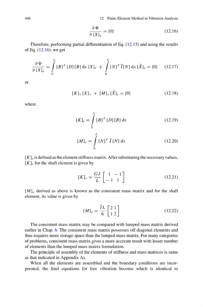
[K ] e is defined as the element stiffness matrix. After substituting the necessary values,
[K ] e for the shaft element is given by
[K ] e =
G J
L
1 − 1
− 1 1
(12.21)
[M] e derived as above is known as the consistent mass matrix and for the shaft
element, its value is given by
[M] e =
I L
6
2 1
1 2
(12.22)
The consistent mass matrix may be compared with lumped mass matrix derived
earlier in Chap. 6. The consistent mass matrix possesses off diagonal elements and
thus requires more storage space than the lumped mass matrix. For many categories
of problems, consistent mass matrix gives a more accurate result with lesser number
of elements than the lumped mass matrix formulation.
The principle of assembly of the elements of stiffness and mass matrices is same
as that indicated in Appendix As.
When all the elements are assembled and the boundary conditions are incorporated, the final equations for free vibration become which is identical to
12 Finite Element Method in Vibration Analysis
∂ ∂
∂ {X } e
= {0}
(12.16)
Therefore, performing partial differentiation of Eq. (12.15) and using the results
of Eq. (12.16), we get
∂ ∂
∂ {X } e
=
L
0
[B]
T
[D] [B] dx {X } e +
L
0
[N ]
T I [N ] dx { ¨
X } e = {0}
(12.17)
or
[K ] e {X } e + [M] e { ¨
X } e = {0}
(12.18)
where
[K ] e =
L
0
[B]
T
[D] [B] dx
(12.19)
[M] e =
L
0
[N ]
T I [N ] dx
(12.20)
[K ] e is defined as the element stiffness matrix. After substituting the necessary values,
[K ] e for the shaft element is given by
[K ] e =
G J
L
1 − 1
− 1 1
(12.21)
[M] e derived as above is known as the consistent mass matrix and for the shaft
element, its value is given by
[M] e =
I L
6
2 1
1 2
(12.22)
The consistent mass matrix may be compared with lumped mass matrix derived
earlier in Chap. 6. The consistent mass matrix possesses off diagonal elements and
thus requires more storage space than the lumped mass matrix. For many categories
of problems, consistent mass matrix gives a more accurate result with lesser number
of elements than the lumped mass matrix formulation.
The principle of assembly of the elements of stiffness and mass matrices is same
as that indicated in Appendix As.
When all the elements are assembled and the boundary conditions are incorporated, the final equations for free vibration become which is identical to