

336
8 Free Vibration Analysis of Continuous Systems
8.9 Orthogonality Properties of Normal Modes
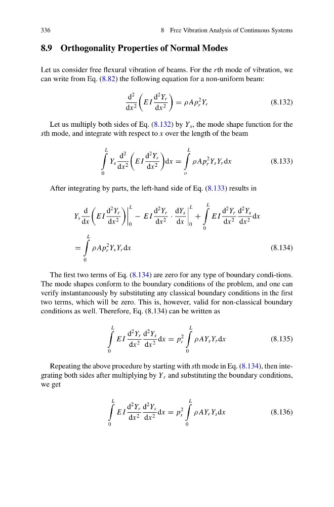
Let us consider free flexural vibration of beams. For the rth mode of vibration, we
can write from Eq. (8.82) the following equation for a non-uniform beam:
d
2
dx 2
E I
d
2 Y r
dx 2
= ρ Ap
2
r Y r
(8.132)
Let us multiply both sides of Eq. (8.132) by Y s , the mode shape function for the
sth mode, and integrate with respect to x over the length of the beam
L
0
Y s
d
2
dx 2
E I
d
2 Y r
dx 2
dx =
L
o
ρ Ap
2
r Y s Y r dx
(8.133)
After integrating by parts, the left-hand side of Eq. (8.133) results in
Y s
d
dx
E I
d
2 Y r
dx 2
L
0
− E I
d
2 Y r
dx 2 ·
dY s
dx
L
0
+
L
0
E I
d
2 Y r
dx 2
d
2 Y s
dx 2 dx
=
L
0
ρ Ap
2
r Y s Y r dx
(8.134)
The first two terms of Eq. (8.134) are zero for any type of boundary condi-tions.
The mode shapes conform to the boundary conditions of the problem, and one can
verify instantaneously by substituting any classical boundary conditions in the first
two terms, which will be zero. This is, however, valid for non-classical boundary
conditions as well. Therefore, Eq. (8.134) can be written as
L
0
E I
d
2 Y r
dx 2
d
2 Y s
dx 2 dx = p
2
r
L
0
ρ AY s Y r dx
(8.135)
Repeating the above procedure by starting with sth mode in Eq. (8.134), then integrating both sides after multiplying by Y r and substituting the boundary conditions,
we get
L
0
E I
d
2 Y r
dx 2
d
2 Y s
dx 2 dx = p
2
s
L
0
ρ AY r Y s dx
(8.136)
8 Free Vibration Analysis of Continuous Systems
8.9 Orthogonality Properties of Normal Modes
Let us consider free flexural vibration of beams. For the rth mode of vibration, we
can write from Eq. (8.82) the following equation for a non-uniform beam:
d
2
dx 2
E I
d
2 Y r
dx 2
= ρ Ap
2
r Y r
(8.132)
Let us multiply both sides of Eq. (8.132) by Y s , the mode shape function for the
sth mode, and integrate with respect to x over the length of the beam
L
0
Y s
d
2
dx 2
E I
d
2 Y r
dx 2
dx =
L
o
ρ Ap
2
r Y s Y r dx
(8.133)
After integrating by parts, the left-hand side of Eq. (8.133) results in
Y s
d
dx
E I
d
2 Y r
dx 2
L
0
− E I
d
2 Y r
dx 2 ·
dY s
dx
L
0
+
L
0
E I
d
2 Y r
dx 2
d
2 Y s
dx 2 dx
=
L
0
ρ Ap
2
r Y s Y r dx
(8.134)
The first two terms of Eq. (8.134) are zero for any type of boundary condi-tions.
The mode shapes conform to the boundary conditions of the problem, and one can
verify instantaneously by substituting any classical boundary conditions in the first
two terms, which will be zero. This is, however, valid for non-classical boundary
conditions as well. Therefore, Eq. (8.134) can be written as
L
0
E I
d
2 Y r
dx 2
d
2 Y s
dx 2 dx = p
2
r
L
0
ρ AY s Y r dx
(8.135)
Repeating the above procedure by starting with sth mode in Eq. (8.134), then integrating both sides after multiplying by Y r and substituting the boundary conditions,
we get
L
0
E I
d
2 Y r
dx 2
d
2 Y s
dx 2 dx = p
2
s
L
0
ρ AY r Y s dx
(8.136)