

7.5 Damping in MDF Systems
273
7.5 Damping in MDF Systems
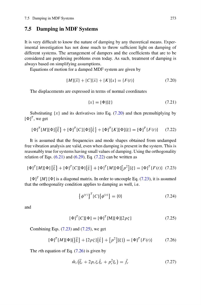
It is very difficult to know the nature of damping by any theoretical means. Experimental investigation has not done much to throw sufficient light on damping of
different systems. The arrangement of dampers and the coefficients that are to be
considered are perplexing problems even today. As such, treatment of damping is
always based on simplifying assumptions.
Equations of motion for a damped MDF system are given by
[M]{ ¨
x} + [C]{ ˙
x} + [K ]{x} = {F(t)}
(7.20)
The displacements are expressed in terms of normal coordinates
{x} = []{ξ }
(7.21)
Substituting {x} and its derivatives into Eq. (7.20) and then premultiplying by
[]
T , we get
[]
T [M][]
¨
ξ
+ []
T [C][]
˙
ξ
+ []
T [K ][]{ξ } = []
T
{F(t)}
(7.22)
It is assumed that the frequencies and mode shapes obtained from undamped
free vibration analysis are valid, even when damping is present in the system. This is
reasonably true for systems having small values of damping. Using the orthogonality
relation of Eqs. (6.21) and (6.29), Eq. (7.22) can be written as
[]
T [M][]
¨
ξ
+ []
T [C][]
˙
ξ
+ []
T [M][]
p
2
{ξ } = []
T
{F(t)} (7.23)
[]
T [M] [] is a diagonal matrix. In order to uncouple Eq. (7.23), it is assumed
that the orthogonality condition applies to damping as well, i.e.
φ
(r )
T [C]
φ
(s)
= {0}
(7.24)
and
[]
T [C][] = []
T [M][][2 pζ ]
(7.25)
Combining Eqs. (7.23) and (7.25), we get
[]
T [M][]
¨
ξ
+ [2 pζ ]
˙
ξ
+
p
2
{ξ }
= []
T
{F(t)}
(7.26)
The rth equation of Eq. (7.26) is given by
¯
m r
¨
ξ r + 2 p r ζ r ˙
ξ r + p
2
r ξ r
= ¯
f r
(7.27)
273
7.5 Damping in MDF Systems
It is very difficult to know the nature of damping by any theoretical means. Experimental investigation has not done much to throw sufficient light on damping of
different systems. The arrangement of dampers and the coefficients that are to be
considered are perplexing problems even today. As such, treatment of damping is
always based on simplifying assumptions.
Equations of motion for a damped MDF system are given by
[M]{ ¨
x} + [C]{ ˙
x} + [K ]{x} = {F(t)}
(7.20)
The displacements are expressed in terms of normal coordinates
{x} = []{ξ }
(7.21)
Substituting {x} and its derivatives into Eq. (7.20) and then premultiplying by
[]
T , we get
[]
T [M][]
¨
ξ
+ []
T [C][]
˙
ξ
+ []
T [K ][]{ξ } = []
T
{F(t)}
(7.22)
It is assumed that the frequencies and mode shapes obtained from undamped
free vibration analysis are valid, even when damping is present in the system. This is
reasonably true for systems having small values of damping. Using the orthogonality
relation of Eqs. (6.21) and (6.29), Eq. (7.22) can be written as
[]
T [M][]
¨
ξ
+ []
T [C][]
˙
ξ
+ []
T [M][]
p
2
{ξ } = []
T
{F(t)} (7.23)
[]
T [M] [] is a diagonal matrix. In order to uncouple Eq. (7.23), it is assumed
that the orthogonality condition applies to damping as well, i.e.
φ
(r )
T [C]
φ
(s)
= {0}
(7.24)
and
[]
T [C][] = []
T [M][][2 pζ ]
(7.25)
Combining Eqs. (7.23) and (7.25), we get
[]
T [M][]
¨
ξ
+ [2 pζ ]
˙
ξ
+
p
2
{ξ }
= []
T
{F(t)}
(7.26)
The rth equation of Eq. (7.26) is given by
¯
m r
¨
ξ r + 2 p r ζ r ˙
ξ r + p
2
r ξ r
= ¯
f r
(7.27)