

7.2 Mode Superposition Method …
265
x 1 (t) =
1.0(P cos ωt)
20,000 × 1.6896 ×
1924.733 − ω 2
r = 1
+
1.0(P cos ωt)
20,000 × 2.9867
14437.2 − ω 2
⎤
⎥
⎥
⎥
⎦
r = 2
+
1.0(P cos ωt)
20,000 × 13.2
27,889 − ω 2
⎤
⎥
⎥
⎥
⎥
⎥
⎥
⎥
⎥
⎦
r = 3
Say
C o =
x 1 (t)
P cos ωt
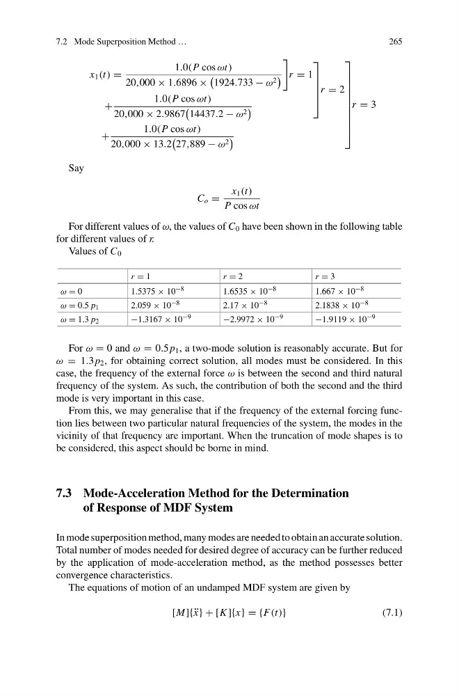
For different values of ω, the values of C 0 have been shown in the following table
for different values of r.
Values of C 0
r = 1
r = 2
r = 3
ω = 0
1.5375 × 10 −8
1.6535 × 10 −8
1.667 × 10 −8
ω = 0.5 p 1
2.059 × 10 −8
2.17 × 10 −8
2.1838 × 10 −8
ω = 1.3 p 2
−1.3167 × 10 −9
−2.9972 × 10 −9
−1.9119 × 10 −9
For ω = 0 and ω = 0.5 p 1 , a two-mode solution is reasonably accurate. But for
ω = 1.3 p 2 , for obtaining correct solution, all modes must be considered. In this
case, the frequency of the external force ω is between the second and third natural
frequency of the system. As such, the contribution of both the second and the third
mode is very important in this case.
From this, we may generalise that if the frequency of the external forcing function lies between two particular natural frequencies of the system, the modes in the
vicinity of that frequency are important. When the truncation of mode shapes is to
be considered, this aspect should be borne in mind.
7.3 Mode-Acceleration Method for the Determination
of Response of MDF System
In mode superposition method, many modes are needed to obtain an accurate solution.
Total number of modes needed for desired degree of accuracy can be further reduced
by the application of mode-acceleration method, as the method possesses better
convergence characteristics.
The equations of motion of an undamped MDF system are given by
[M]{ ¨
x} + [K ]{x} = {F(t)}
(7.1)
265
x 1 (t) =
1.0(P cos ωt)
20,000 × 1.6896 ×
1924.733 − ω 2
r = 1
+
1.0(P cos ωt)
20,000 × 2.9867
14437.2 − ω 2
⎤
⎥
⎥
⎥
⎦
r = 2
+
1.0(P cos ωt)
20,000 × 13.2
27,889 − ω 2
⎤
⎥
⎥
⎥
⎥
⎥
⎥
⎥
⎥
⎦
r = 3
Say
C o =
x 1 (t)
P cos ωt
For different values of ω, the values of C 0 have been shown in the following table
for different values of r.
Values of C 0
r = 1
r = 2
r = 3
ω = 0
1.5375 × 10 −8
1.6535 × 10 −8
1.667 × 10 −8
ω = 0.5 p 1
2.059 × 10 −8
2.17 × 10 −8
2.1838 × 10 −8
ω = 1.3 p 2
−1.3167 × 10 −9
−2.9972 × 10 −9
−1.9119 × 10 −9
For ω = 0 and ω = 0.5 p 1 , a two-mode solution is reasonably accurate. But for
ω = 1.3 p 2 , for obtaining correct solution, all modes must be considered. In this
case, the frequency of the external force ω is between the second and third natural
frequency of the system. As such, the contribution of both the second and the third
mode is very important in this case.
From this, we may generalise that if the frequency of the external forcing function lies between two particular natural frequencies of the system, the modes in the
vicinity of that frequency are important. When the truncation of mode shapes is to
be considered, this aspect should be borne in mind.
7.3 Mode-Acceleration Method for the Determination
of Response of MDF System
In mode superposition method, many modes are needed to obtain an accurate solution.
Total number of modes needed for desired degree of accuracy can be further reduced
by the application of mode-acceleration method, as the method possesses better
convergence characteristics.
The equations of motion of an undamped MDF system are given by
[M]{ ¨
x} + [K ]{x} = {F(t)}
(7.1)