

6.22 Lagrange’s Equation
257
6.19 From the solution of Prob. 6.5, show that the normal modes are mutually
orthogonal.
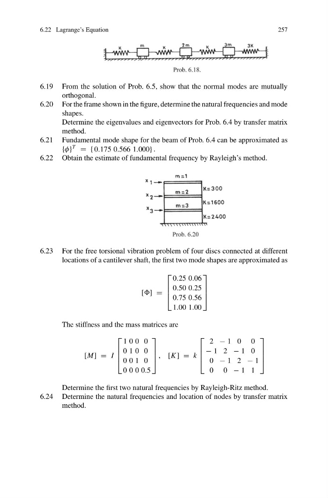
6.20 For the frame shown in the figure, determine the natural frequencies and mode
shapes.
Determine the eigenvalues and eigenvectors for Prob. 6.4 by transfer matrix
method.
6.21 Fundamental mode shape for the beam of Prob. 6.4 can be approximated as
{φ}
T
= {0.175 0.566 1.000} .
6.22 Obtain the estimate of fundamental frequency by Rayleigh’s method.
6.23 For the free torsional vibration problem of four discs connected at different
locations of a cantilever shaft, the first two mode shapes are approximated as
[] =
⎡
⎢
⎢
⎣
0.25 0.06
0.50 0.25
0.75 0.56
1.00 1.00
⎤
⎥
⎥
⎦
The stiffness and the mass matrices are
[M] = I
⎡
⎢
⎢
⎣
1 0 0 0
0 1 0 0
0 0 1 0
0 0 0 0.5
⎤
⎥
⎥
⎦ , [K ] = k
⎡
⎢
⎢
⎣
2 − 1 0 0
− 1 2 − 1 0
0 − 1 2 − 1
0 0 − 1 1
⎤
⎥
⎥
⎦
Determine the first two natural frequencies by Rayleigh-Ritz method.
6.24 Determine the natural frequencies and location of nodes by transfer matrix
method.
257
6.19 From the solution of Prob. 6.5, show that the normal modes are mutually
orthogonal.
6.20 For the frame shown in the figure, determine the natural frequencies and mode
shapes.
Determine the eigenvalues and eigenvectors for Prob. 6.4 by transfer matrix
method.
6.21 Fundamental mode shape for the beam of Prob. 6.4 can be approximated as
{φ}
T
= {0.175 0.566 1.000} .
6.22 Obtain the estimate of fundamental frequency by Rayleigh’s method.
6.23 For the free torsional vibration problem of four discs connected at different
locations of a cantilever shaft, the first two mode shapes are approximated as
[] =
⎡
⎢
⎢
⎣
0.25 0.06
0.50 0.25
0.75 0.56
1.00 1.00
⎤
⎥
⎥
⎦
The stiffness and the mass matrices are
[M] = I
⎡
⎢
⎢
⎣
1 0 0 0
0 1 0 0
0 0 1 0
0 0 0 0.5
⎤
⎥
⎥
⎦ , [K ] = k
⎡
⎢
⎢
⎣
2 − 1 0 0
− 1 2 − 1 0
0 − 1 2 − 1
0 0 − 1 1
⎤
⎥
⎥
⎦
Determine the first two natural frequencies by Rayleigh-Ritz method.
6.24 Determine the natural frequencies and location of nodes by transfer matrix
method.