

6.21 Component Mode Synthesis Method
251
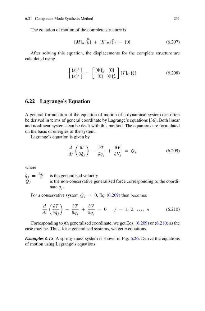
The equation of motion of the complete structure is
[M] R { ¨
ξ } + [K ] R {ξ } = {0}
(6.207)
After solving this equation, the displacements for the complete structure are
calculated using
{x}
1
{x}
2
=
[]
1
N [0]
[0] []
2
N
[T ] C {ξ }
(6.208)
6.22 Lagrange’s Equation
A general formulation of the equation of motion of a dynamical system can often
be derived in terms of general coordinate by Lagrange’s equations [36]. Both linear
and nonlinear systems can be dealt with this method. The equations are formulated
on the basis of energies of the system.
Lagrange’s equation is given by
d
dt
∂t
∂ ˙
q j
−
∂ T
∂q j
+
∂ V
∂ V j
= Q j
(6.209)
where
˙
q j =
∂q j
∂t
is the generalised velocity.
Q j
is the non-conservative generalised force corresponding to the coordinate q j .
For a conservative system Q j = 0, Eq. (6.209) then becomes
d
dt
∂ T
∂ ˙
q j
−
∂ T
∂q j
+
∂ V
∂q j
= 0
j = 1, 2, . . . , n
(6.210)
Corresponding to jth generalised coordinate, we get Eqs. (6.209) or (6.210) as the
case may be. Thus, for n generalised systems, we get n equations.
Examples 6.15 A spring–mass system is shown in Fig. 6.26. Derive the equations
of motion using Lagrange’s equations.
251
The equation of motion of the complete structure is
[M] R { ¨
ξ } + [K ] R {ξ } = {0}
(6.207)
After solving this equation, the displacements for the complete structure are
calculated using
{x}
1
{x}
2
=
[]
1
N [0]
[0] []
2
N
[T ] C {ξ }
(6.208)
6.22 Lagrange’s Equation
A general formulation of the equation of motion of a dynamical system can often
be derived in terms of general coordinate by Lagrange’s equations [36]. Both linear
and nonlinear systems can be dealt with this method. The equations are formulated
on the basis of energies of the system.
Lagrange’s equation is given by
d
dt
∂t
∂ ˙
q j
−
∂ T
∂q j
+
∂ V
∂ V j
= Q j
(6.209)
where
˙
q j =
∂q j
∂t
is the generalised velocity.
Q j
is the non-conservative generalised force corresponding to the coordinate q j .
For a conservative system Q j = 0, Eq. (6.209) then becomes
d
dt
∂ T
∂ ˙
q j
−
∂ T
∂q j
+
∂ V
∂q j
= 0
j = 1, 2, . . . , n
(6.210)
Corresponding to jth generalised coordinate, we get Eqs. (6.209) or (6.210) as the
case may be. Thus, for n generalised systems, we get n equations.
Examples 6.15 A spring–mass system is shown in Fig. 6.26. Derive the equations
of motion using Lagrange’s equations.