

6.21 Component Mode Synthesis Method
245
where subscript I refers to internal nodes and subscript B refers to boundary nodes
which are common to two or more substructures at the boundary.
Using Eqs. (6.28), (6.157) is rewritten
{x}
s
=
{x} I
{x} B
=
[] N [] C
[0] [I ]
{ξ } N
{x} B
(6.158)
or,
{x}
s
= [T ] s {ξ } s
(6.159)
Considering interface boundaries fixed, an eigensolution of the following equation
will give [] N matrix
( [K ] I I − p
2
[M] I I ) {} I = {0}
(6.160)
[K ] I I is the stiffness matrix found by internal nodes (without considering
boundary nodes). Similarly, [M] I I is the appropriate portion of [M]
S . [] N are
general coordinates related to the natural modes of the substructure.
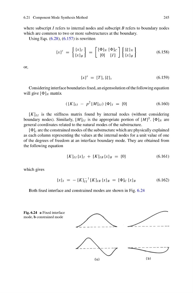
[] c are the constrained modes of the substructure which are physically explained
as each column representing the values at the internal nodes for a unit value of one
of the degrees of freedom at an interface boundary mode. They are obtained from
the following equation
[K ] I I {x} I + [K ] I B {x} B = {0}
(6.161)
which gives
{x} I = − [K ]
− 1
I I [K ] I B {x} B = [] C {x} B
(6.162)
Both fixed interface and constrained modes are shown in Fig. 6.24
Fig. 6.24 a Fixed interface
mode, b constrained mode
245
where subscript I refers to internal nodes and subscript B refers to boundary nodes
which are common to two or more substructures at the boundary.
Using Eqs. (6.28), (6.157) is rewritten
{x}
s
=
{x} I
{x} B
=
[] N [] C
[0] [I ]
{ξ } N
{x} B
(6.158)
or,
{x}
s
= [T ] s {ξ } s
(6.159)
Considering interface boundaries fixed, an eigensolution of the following equation
will give [] N matrix
( [K ] I I − p
2
[M] I I ) {} I = {0}
(6.160)
[K ] I I is the stiffness matrix found by internal nodes (without considering
boundary nodes). Similarly, [M] I I is the appropriate portion of [M]
S . [] N are
general coordinates related to the natural modes of the substructure.
[] c are the constrained modes of the substructure which are physically explained
as each column representing the values at the internal nodes for a unit value of one
of the degrees of freedom at an interface boundary mode. They are obtained from
the following equation
[K ] I I {x} I + [K ] I B {x} B = {0}
(6.161)
which gives
{x} I = − [K ]
− 1
I I [K ] I B {x} B = [] C {x} B
(6.162)
Both fixed interface and constrained modes are shown in Fig. 6.24
Fig. 6.24 a Fixed interface
mode, b constrained mode