

6.20 Reduction Methods for Dynamic Analysis
241
[H ] =
[I ]
[W ]
(6.147)
From Eq. (6.146), we get
δ {x}
T
= δ {x}
T
r [H ]
T
(6.148)
Premultiplying both sides of Eq. (6.144) by δ {x}
T and using Eq. (6.148) yields
δ {x}
T
r ( [H ]
T
[M] [H ] { ¨
x} r + [H ]
T
[C] [H ] { ˙
x} r
[H ]
T
[K ] [H ] {x} r ) = δ {x}
T
r [H ]
T
{F (t) }
(6.149)
From Eq. (6.149), we get
[M] red { ¨
x} r + [C] red { ˙
x} r + [K ] red {x} r = {F} red
(6.150)
where
[M] red = [H ]
T
[M] [H ], [C] red = [H ]
T
[C] [H ]
[K ] red = [H ]
T
[K ] [H ] and {F} red = [H ]
T
{F}
(6.151)
Combining Eqs. (6.147) and (6.151) yields
[M] red = [M] rr + [W ]
T
[M] ir + [M] ri [W ] + [W ]
T
[M] ii [W ] (6.152a)
[C] red = [C] rr + [W ]
T
[C] ir + [C] ri [W ] + [W ]
T
[C] ii [W ]
(6.152b)
[K ] red = [K ] rr + [W ]
T
[K ] ir
(6.152c)
{F} red = {F} r + [W ]
T
{R} i
(6.152d)
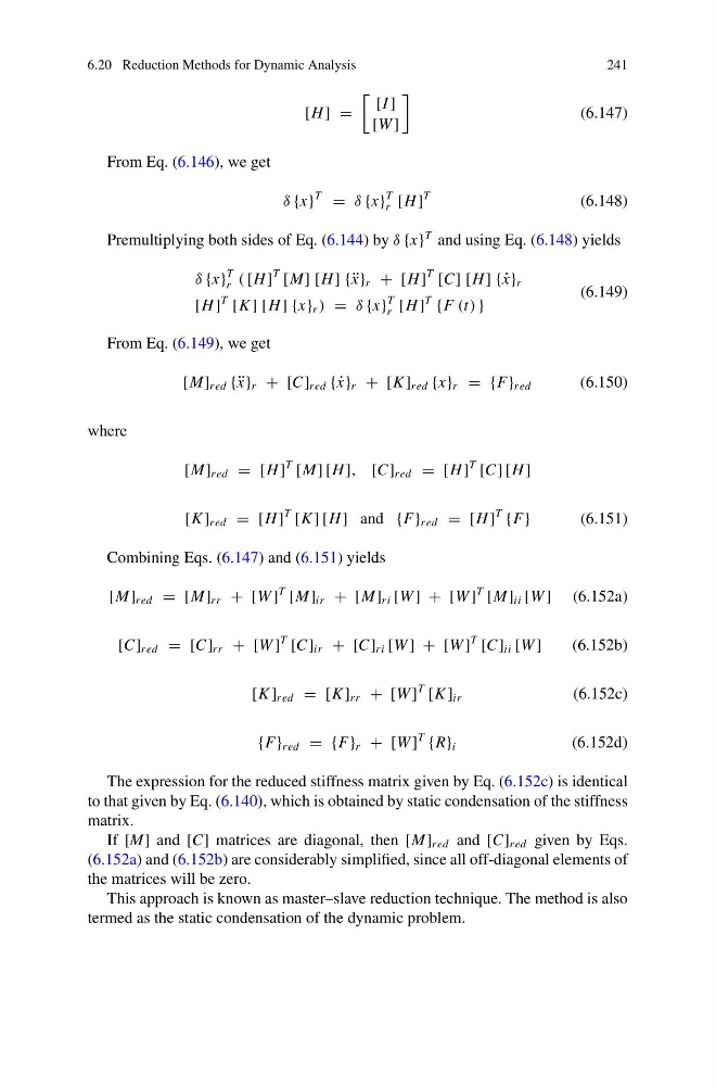
The expression for the reduced stiffness matrix given by Eq. (6.152c) is identical
to that given by Eq. (6.140), which is obtained by static condensation of the stiffness
matrix.
If [M] and [C] matrices are diagonal, then [M] red and [C] red given by Eqs.
(6.152a) and (6.152b) are considerably simplified, since all off-diagonal elements of
the matrices will be zero.
This approach is known as master–slave reduction technique. The method is also
termed as the static condensation of the dynamic problem.
241
[H ] =
[I ]
[W ]
(6.147)
From Eq. (6.146), we get
δ {x}
T
= δ {x}
T
r [H ]
T
(6.148)
Premultiplying both sides of Eq. (6.144) by δ {x}
T and using Eq. (6.148) yields
δ {x}
T
r ( [H ]
T
[M] [H ] { ¨
x} r + [H ]
T
[C] [H ] { ˙
x} r
[H ]
T
[K ] [H ] {x} r ) = δ {x}
T
r [H ]
T
{F (t) }
(6.149)
From Eq. (6.149), we get
[M] red { ¨
x} r + [C] red { ˙
x} r + [K ] red {x} r = {F} red
(6.150)
where
[M] red = [H ]
T
[M] [H ], [C] red = [H ]
T
[C] [H ]
[K ] red = [H ]
T
[K ] [H ] and {F} red = [H ]
T
{F}
(6.151)
Combining Eqs. (6.147) and (6.151) yields
[M] red = [M] rr + [W ]
T
[M] ir + [M] ri [W ] + [W ]
T
[M] ii [W ] (6.152a)
[C] red = [C] rr + [W ]
T
[C] ir + [C] ri [W ] + [W ]
T
[C] ii [W ]
(6.152b)
[K ] red = [K ] rr + [W ]
T
[K ] ir
(6.152c)
{F} red = {F} r + [W ]
T
{R} i
(6.152d)
The expression for the reduced stiffness matrix given by Eq. (6.152c) is identical
to that given by Eq. (6.140), which is obtained by static condensation of the stiffness
matrix.
If [M] and [C] matrices are diagonal, then [M] red and [C] red given by Eqs.
(6.152a) and (6.152b) are considerably simplified, since all off-diagonal elements of
the matrices will be zero.
This approach is known as master–slave reduction technique. The method is also
termed as the static condensation of the dynamic problem.