

6.20 Reduction Methods for Dynamic Analysis
239
6.20.1 Static Condensation
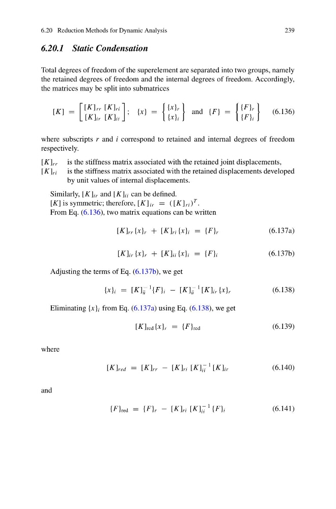
Total degrees of freedom of the superelement are separated into two groups, namely
the retained degrees of freedom and the internal degrees of freedom. Accordingly,
the matrices may be split into submatrices
[K ] =
[K ] rr [K ] ri
[K ] ir [K ] ii
; {x} =
{x} r
{x} i
and {F} =
{F} r
{F} i
(6.136)
where subscripts r and i correspond to retained and internal degrees of freedom
respectively.
[K ] rr is the stiffness matrix associated with the retained joint displacements,
[K ] ri is the stiffness matrix associated with the retained displacements developed
by unit values of internal displacements.
Similarly, [K ] ir and [K ] ii can be defined.
[K] is symmetric; therefore, [K ] ir = ( [K ] ri )
T .
From Eq. (6.136), two matrix equations can be written
[K ] rr {x} r + [K ] ri {x} i = {F} r
(6.137a)
[K ] ir {x} r + [K ] ii {x} i = {F} i
(6.137b)
Adjusting the terms of Eq. (6.137b), we get
{x} i = [K ]
− 1
¨
u {F} i − [K ]
− 1
¨
u [K ] ir {x} r
(6.138)
Eliminating {x} i from Eq. (6.137a) using Eq. (6.138), we get
[K ] red {x} r = {F} red
(6.139)
where
[K ] red = [K ] rr − [K ] ri [K ]
− 1
ii [K ] ir
(6.140)
and
{F} red = {F} r − [K ] ri [K ]
− 1
ii {F} i
(6.141)
239
6.20.1 Static Condensation
Total degrees of freedom of the superelement are separated into two groups, namely
the retained degrees of freedom and the internal degrees of freedom. Accordingly,
the matrices may be split into submatrices
[K ] =
[K ] rr [K ] ri
[K ] ir [K ] ii
; {x} =
{x} r
{x} i
and {F} =
{F} r
{F} i
(6.136)
where subscripts r and i correspond to retained and internal degrees of freedom
respectively.
[K ] rr is the stiffness matrix associated with the retained joint displacements,
[K ] ri is the stiffness matrix associated with the retained displacements developed
by unit values of internal displacements.
Similarly, [K ] ir and [K ] ii can be defined.
[K] is symmetric; therefore, [K ] ir = ( [K ] ri )
T .
From Eq. (6.136), two matrix equations can be written
[K ] rr {x} r + [K ] ri {x} i = {F} r
(6.137a)
[K ] ir {x} r + [K ] ii {x} i = {F} i
(6.137b)
Adjusting the terms of Eq. (6.137b), we get
{x} i = [K ]
− 1
¨
u {F} i − [K ]
− 1
¨
u [K ] ir {x} r
(6.138)
Eliminating {x} i from Eq. (6.137a) using Eq. (6.138), we get
[K ] red {x} r = {F} red
(6.139)
where
[K ] red = [K ] rr − [K ] ri [K ]
− 1
ii [K ] ir
(6.140)
and
{F} red = {F} r − [K ] ri [K ]
− 1
ii {F} i
(6.141)