

226
6 Free Vibration of Multiple Degrees of Freedom System
{φ } = {φ } − α {φ
(1)
}
(6.94)
and the value of α is such that {φ} is orthogonal to {φ
(1)
}. Therefore,
{φ
(1)
}
T
[M] {φ} = {0 }
or
{φ
(1)
}
T
[M] [{φ} − α {φ
(1)
}] = {0}
or
α =
{φ
(1)
}
T
[M] {φ}
{φ (1) } T [M] {φ (1) }
{φ}
(6.95)
Substituting α from Eq. (6.95) into Eq. (6.94), we obtain
{φ} = {φ} −
{φ
(1)
} {φ
(1)
}
T
[M]
{φ (1) } T [M] {φ (1) }
{φ}
(6.96)
One can now use {φ} as the starting vector instead of {φ}, and the convergence to
the second mode is thus achieved.
In order to determine {φ
(3)
} by inverse iteration, we must remove both {φ
(1)
} and
{φ
(2)
} as shown below
{φ} = {φ } − α 1 {φ
(1)
} − α 2 {φ
(2)
}
(6.97)
In order to determine α 1 and α 2 , the orthogonality relationships can be used as
demonstrated above. The procedure may be repeated for other higher modes.
However, if the iteration is carried out with {φ}, then due to round-off errors,
{φ
(1)
} may be reintroduced in the trial vectors. Therefore, the modification as given
by Eq. (6.83) or (6.96) is to be made for each cycle of iteration.
It is more convenient to work on a modified matrix
[D] {φ} = [D]
[I ] −
{φ
(1)
}
T
{φ
(1)
} [M]
{φ (1) } T [M] {φ (1) }
{φ}
(6.98)
where [S] = [I ] −
{φ
(1) }
T {φ
(1) } [M]
{φ (1) } T [M] {φ (1) }
.
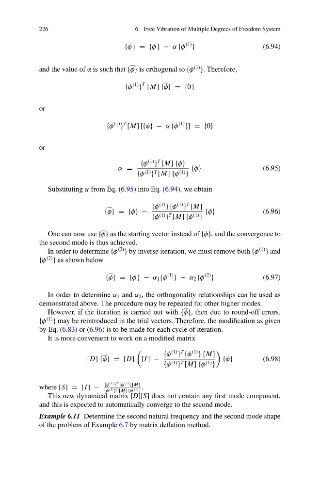
This new dynamical matrix [D][S] does not contain any first mode component,
and this is expected to automatically converge to the second mode.
Example 6.11 Determine the second natural frequency and the second mode shape
of the problem of Example 6.7 by matrix deflation method.
6 Free Vibration of Multiple Degrees of Freedom System
{φ } = {φ } − α {φ
(1)
}
(6.94)
and the value of α is such that {φ} is orthogonal to {φ
(1)
}. Therefore,
{φ
(1)
}
T
[M] {φ} = {0 }
or
{φ
(1)
}
T
[M] [{φ} − α {φ
(1)
}] = {0}
or
α =
{φ
(1)
}
T
[M] {φ}
{φ (1) } T [M] {φ (1) }
{φ}
(6.95)
Substituting α from Eq. (6.95) into Eq. (6.94), we obtain
{φ} = {φ} −
{φ
(1)
} {φ
(1)
}
T
[M]
{φ (1) } T [M] {φ (1) }
{φ}
(6.96)
One can now use {φ} as the starting vector instead of {φ}, and the convergence to
the second mode is thus achieved.
In order to determine {φ
(3)
} by inverse iteration, we must remove both {φ
(1)
} and
{φ
(2)
} as shown below
{φ} = {φ } − α 1 {φ
(1)
} − α 2 {φ
(2)
}
(6.97)
In order to determine α 1 and α 2 , the orthogonality relationships can be used as
demonstrated above. The procedure may be repeated for other higher modes.
However, if the iteration is carried out with {φ}, then due to round-off errors,
{φ
(1)
} may be reintroduced in the trial vectors. Therefore, the modification as given
by Eq. (6.83) or (6.96) is to be made for each cycle of iteration.
It is more convenient to work on a modified matrix
[D] {φ} = [D]
[I ] −
{φ
(1)
}
T
{φ
(1)
} [M]
{φ (1) } T [M] {φ (1) }
{φ}
(6.98)
where [S] = [I ] −
{φ
(1) }
T {φ
(1) } [M]
{φ (1) } T [M] {φ (1) }
.
This new dynamical matrix [D][S] does not contain any first mode component,
and this is expected to automatically converge to the second mode.
Example 6.11 Determine the second natural frequency and the second mode shape
of the problem of Example 6.7 by matrix deflation method.