

6.12 Stodola’s Method
225
f 21 = f 12 = f 32 = f 23 =
3.67 L
3
256 E I
Therefore,
[F] =
L
3
256 E I
⎡
⎣
3.00 3.67 2.33
3.67 5.33 3.67
2.33 3.67 3.00
⎤
⎦
[D] = [F] [M] =
M L
3
1024 E I
⎡
⎣
3.00 3.67 2.33
3.67 5.33 3.67
2.33 3.67 3.00
⎤
⎦
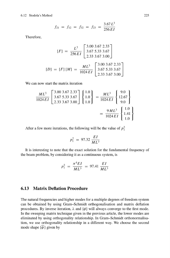
We can now start the matrix iteration
M L
3
1024 E I
⎡
⎣
3.00 3.67 2.33
3.67 5.33 3.67
2.33 3.67 3.00
⎤
⎦
⎧
⎨
⎩
1.0
1.0
1.0
⎫
⎬
⎭
=
M L
3
1024 E I
⎧
⎨
⎩
9.0
12.67
9.0
⎫
⎬
⎭
=
9 M L
3
1024 E I
⎧
⎨
⎩
1.0
1.41
1.0
⎫
⎬
⎭
After a few more iterations, the following will be the value of p
2
1
p
2
1 = 97.32
E I
M L 3
It is interesting to note that the exact solution for the fundamental frequency of
the beam problem, by considering it as a continuous system, is
p
2
1 =
π
4 E I
M L 3 = 97.41
E I
M L 3
6.13 Matrix Deflation Procedure
The natural frequencies and higher modes for a multiple degrees of freedom system
can be obtained by using Gram–Schmidt orthogonalisation and matrix deflation
procedures. By inverse iteration, λ and {φ} will always converge to the first mode.
In the sweeping matrix technique given in the previous article, the lower modes are
eliminated by using orthogonality relationship. In Gram–Schmidt orthonormalisation, we use orthogonality relationship in a different way. We choose the second
mode shape {φ } given by
225
f 21 = f 12 = f 32 = f 23 =
3.67 L
3
256 E I
Therefore,
[F] =
L
3
256 E I
⎡
⎣
3.00 3.67 2.33
3.67 5.33 3.67
2.33 3.67 3.00
⎤
⎦
[D] = [F] [M] =
M L
3
1024 E I
⎡
⎣
3.00 3.67 2.33
3.67 5.33 3.67
2.33 3.67 3.00
⎤
⎦
We can now start the matrix iteration
M L
3
1024 E I
⎡
⎣
3.00 3.67 2.33
3.67 5.33 3.67
2.33 3.67 3.00
⎤
⎦
⎧
⎨
⎩
1.0
1.0
1.0
⎫
⎬
⎭
=
M L
3
1024 E I
⎧
⎨
⎩
9.0
12.67
9.0
⎫
⎬
⎭
=
9 M L
3
1024 E I
⎧
⎨
⎩
1.0
1.41
1.0
⎫
⎬
⎭
After a few more iterations, the following will be the value of p
2
1
p
2
1 = 97.32
E I
M L 3
It is interesting to note that the exact solution for the fundamental frequency of
the beam problem, by considering it as a continuous system, is
p
2
1 =
π
4 E I
M L 3 = 97.41
E I
M L 3
6.13 Matrix Deflation Procedure
The natural frequencies and higher modes for a multiple degrees of freedom system
can be obtained by using Gram–Schmidt orthogonalisation and matrix deflation
procedures. By inverse iteration, λ and {φ} will always converge to the first mode.
In the sweeping matrix technique given in the previous article, the lower modes are
eliminated by using orthogonality relationship. In Gram–Schmidt orthonormalisation, we use orthogonality relationship in a different way. We choose the second
mode shape {φ } given by