

6.10 Transfer Matrix Method
211
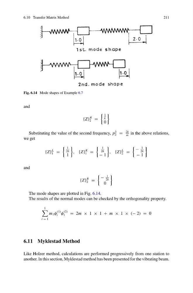
Fig. 6.14 Mode shapes of Example 6.7
and
{Z }
R
2 =
1
k
0
Substituting the value of the second frequency, p
2
2 =
2k
m
in the above relations,
we get
{Z }
L
1 =
1
2k
1
, {Z }
R
1 =
1
2k
− 1
, {Z }
L
2 =
−
1
2k
− 1
and
{Z }
R
2 =
−
1
2k
0
The mode shapes are plotted in Fig. 6.14.
The results of the normal modes can be checked by the orthogonality property.
1
i = 1
m 1 φ
(1)
i φ
(2)
1
= 2m × 1 × 1 + m × 1 × (− 2) = 0
6.11 Myklestad Method
Like Holzer method, calculations are performed progressively from one station to
another. In this section, Myklestad method has been presented for the vibrating beam.
211
Fig. 6.14 Mode shapes of Example 6.7
and
{Z }
R
2 =
1
k
0
Substituting the value of the second frequency, p
2
2 =
2k
m
in the above relations,
we get
{Z }
L
1 =
1
2k
1
, {Z }
R
1 =
1
2k
− 1
, {Z }
L
2 =
−
1
2k
− 1
and
{Z }
R
2 =
−
1
2k
0
The mode shapes are plotted in Fig. 6.14.
The results of the normal modes can be checked by the orthogonality property.
1
i = 1
m 1 φ
(1)
i φ
(2)
1
= 2m × 1 × 1 + m × 1 × (− 2) = 0
6.11 Myklestad Method
Like Holzer method, calculations are performed progressively from one station to
another. In this section, Myklestad method has been presented for the vibrating beam.