

6.9 Holzer Method
201
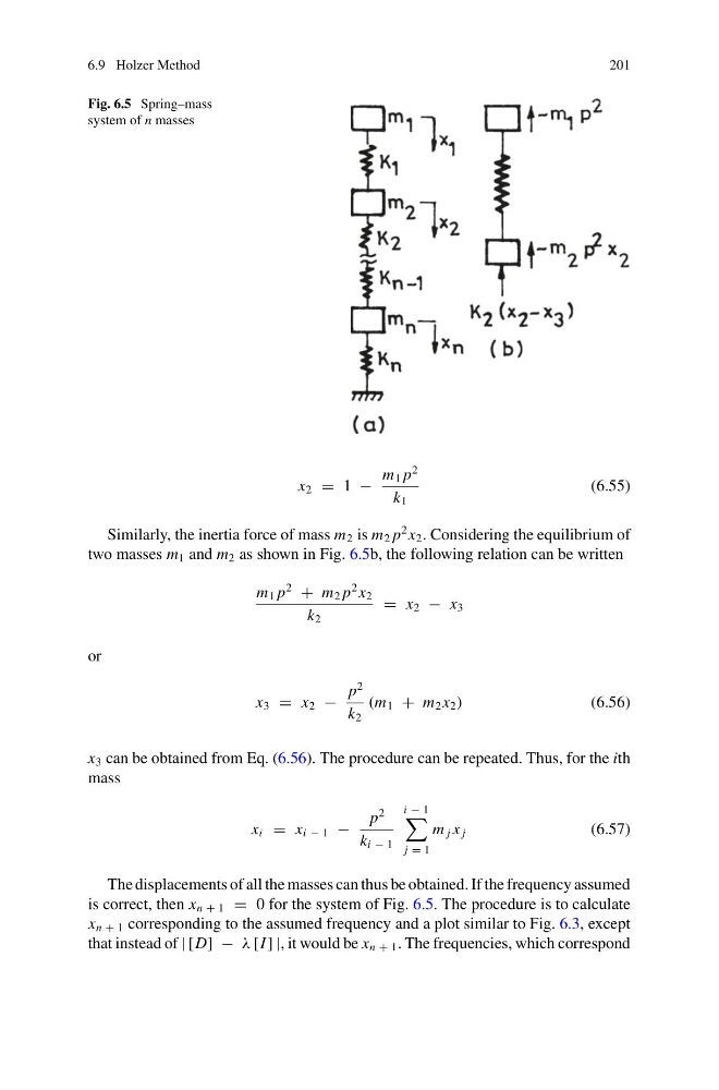
Fig. 6.5 Spring–mass
system of n masses
x 2 = 1 −
m 1 p
2
k 1
(6.55)
Similarly, the inertia force of mass m 2 is m 2 p
2 x 2 . Considering the equilibrium of
two masses m 1 and m 2 as shown in Fig. 6.5b, the following relation can be written
m 1 p
2
+ m 2 p
2 x 2
k 2
= x 2 − x 3
or
x 3 = x 2 −
p
2
k 2
(m 1 + m 2 x 2 )
(6.56)
x 3 can be obtained from Eq. (6.56). The procedure can be repeated. Thus, for the ith
mass
x i = x i − 1 −
p
2
k i − 1
i − 1
j = 1
m j x j
(6.57)
The displacements of all the masses can thus be obtained. If the frequency assumed
is correct, then x n + 1 = 0 for the system of Fig. 6.5. The procedure is to calculate
x n + 1 corresponding to the assumed frequency and a plot similar to Fig. 6.3, except
that instead of | [D] − λ [I ] |, it would be x n + 1 . The frequencies, which correspond
201
Fig. 6.5 Spring–mass
system of n masses
x 2 = 1 −
m 1 p
2
k 1
(6.55)
Similarly, the inertia force of mass m 2 is m 2 p
2 x 2 . Considering the equilibrium of
two masses m 1 and m 2 as shown in Fig. 6.5b, the following relation can be written
m 1 p
2
+ m 2 p
2 x 2
k 2
= x 2 − x 3
or
x 3 = x 2 −
p
2
k 2
(m 1 + m 2 x 2 )
(6.56)
x 3 can be obtained from Eq. (6.56). The procedure can be repeated. Thus, for the ith
mass
x i = x i − 1 −
p
2
k i − 1
i − 1
j = 1
m j x j
(6.57)
The displacements of all the masses can thus be obtained. If the frequency assumed
is correct, then x n + 1 = 0 for the system of Fig. 6.5. The procedure is to calculate
x n + 1 corresponding to the assumed frequency and a plot similar to Fig. 6.3, except
that instead of | [D] − λ [I ] |, it would be x n + 1 . The frequencies, which correspond