

6.7 Eigenvalue Solution Techniques
197
where {φ
(1)
} is the mode shape for the first mode and so is the definition of
{φ
(2)
}, {φ
(3)
}, etc. It may be noted that [] is a square matrix of order n × n.
Further, from the orthogonality properties given by Eqs. (6.19) and (6.20), [] is
a square diagonal matrix containing p
2 values in the diagonal elements.
Due to transformations of the types given by Eqs. (6.43) and (6.44), this method
of solution requires storage of large matrices.
Since [] the mode shape matrix is unique, it can be constructed by iteration.
Basically, the method involves the reduction of [K] and [M] into diagonal form,
using successive premultiplication and post-multiplication of suitable matrices. A
sequence of matrix transformations is thus obtained for the final evaluation. In this
method, unless all the eigenvalues and eigenvectors are evaluated, the final output
cannot be obtained.
Earlier transformation methods are due to Jacobi, Givens and Householder. It is
very difficult to obtain stable methods, which are reliable as well as convergent for
unsymmetric eigenvalue problems. The Eberline extension of Jacobi’s transformation
method is noted for its lack of universal stability. As such, attempts have been made
to develop stable forms of the Eberline method. QR transformation method is one
of the methods falling in this group, in which the stiffness matrix [K] is transformed
into tri-diagonal form, and then, rotation matrices are employed.
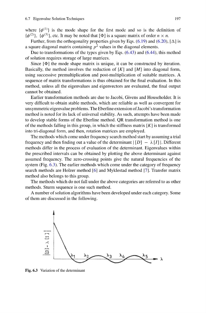
The methods which come under frequency search method start by assuming a trial
frequency and then finding out a value of the determinant | [D] − λ [I ] |. Different
methods differ in the process of evaluation of the determinant. Eigenvalues within
the prescribed intervals can be obtained by plotting the above determinant against
assumed frequency. The zero-crossing points give the natural frequencies of the
system (Fig. 6.3). The earlier methods which come under the category of frequency
search methods are Holzer method [6] and Myklestad method [7]. Transfer matrix
method also belongs to this group.
The methods which do not fall under the above categories are referred to as other
methods. Sturm sequence is one such method.
A number of solution algorithms have been developed under each category. Some
of them are discussed in the following.
Fig. 6.3 Variation of the determinant
197
where {φ
(1)
} is the mode shape for the first mode and so is the definition of
{φ
(2)
}, {φ
(3)
}, etc. It may be noted that [] is a square matrix of order n × n.
Further, from the orthogonality properties given by Eqs. (6.19) and (6.20), [] is
a square diagonal matrix containing p
2 values in the diagonal elements.
Due to transformations of the types given by Eqs. (6.43) and (6.44), this method
of solution requires storage of large matrices.
Since [] the mode shape matrix is unique, it can be constructed by iteration.
Basically, the method involves the reduction of [K] and [M] into diagonal form,
using successive premultiplication and post-multiplication of suitable matrices. A
sequence of matrix transformations is thus obtained for the final evaluation. In this
method, unless all the eigenvalues and eigenvectors are evaluated, the final output
cannot be obtained.
Earlier transformation methods are due to Jacobi, Givens and Householder. It is
very difficult to obtain stable methods, which are reliable as well as convergent for
unsymmetric eigenvalue problems. The Eberline extension of Jacobi’s transformation
method is noted for its lack of universal stability. As such, attempts have been made
to develop stable forms of the Eberline method. QR transformation method is one
of the methods falling in this group, in which the stiffness matrix [K] is transformed
into tri-diagonal form, and then, rotation matrices are employed.
The methods which come under frequency search method start by assuming a trial
frequency and then finding out a value of the determinant | [D] − λ [I ] |. Different
methods differ in the process of evaluation of the determinant. Eigenvalues within
the prescribed intervals can be obtained by plotting the above determinant against
assumed frequency. The zero-crossing points give the natural frequencies of the
system (Fig. 6.3). The earlier methods which come under the category of frequency
search methods are Holzer method [6] and Myklestad method [7]. Transfer matrix
method also belongs to this group.
The methods which do not fall under the above categories are referred to as other
methods. Sturm sequence is one such method.
A number of solution algorithms have been developed under each category. Some
of them are discussed in the following.
Fig. 6.3 Variation of the determinant