

6.4 Orthogonality Relationship
189
Comparing Eq. (6.18) with the first of Eq. (6.17), we get for r = s,
{φ
(s)
}
T
[M] {φ
(r )
} = {0}
(6.19)
and
{φ
(s)
}
T
[K ] {φ
(r )
} = {0}
(6.20)
If [M] is a diagonal matrix, Eq. (6.20) can be written as
n
i = 1
m i φ
(r )
i φ
(s)
i
= 0
(6.21)
Equations (6.19)–(6.21) are known as orthogonality relationship. As we shall see
later in this chapter, this relationship is used for solving eigenvalue problems, as also
for the treatment of forced vibration. The orthogonality relationship is a fundamental
property of MDF systems.
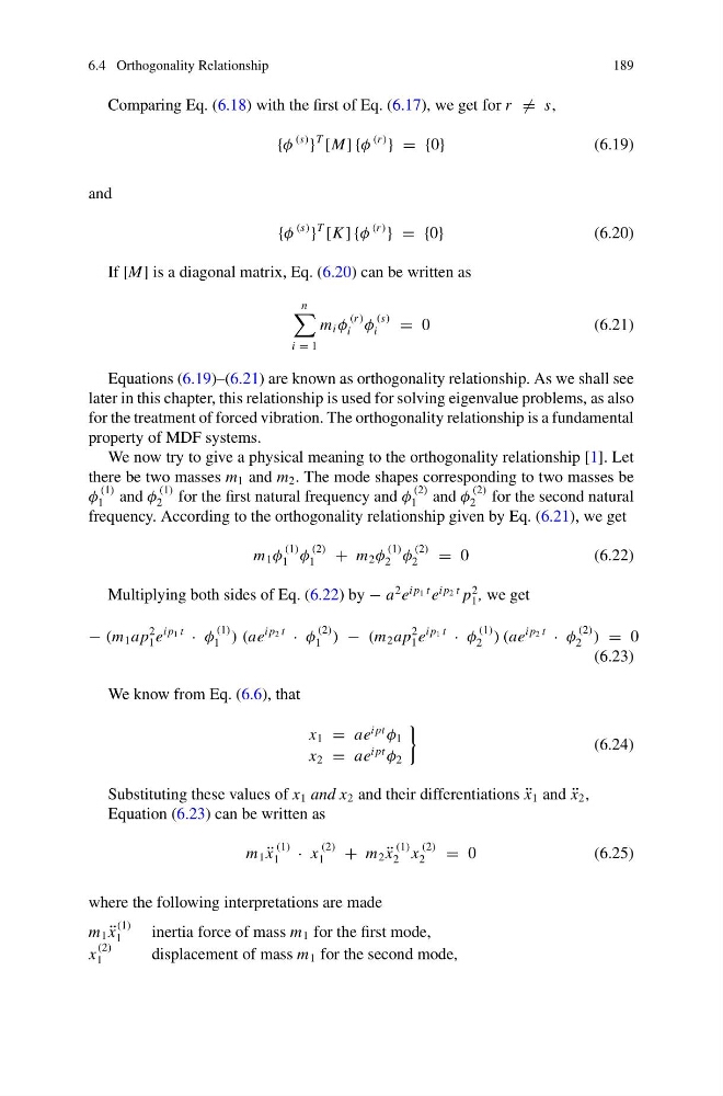
We now try to give a physical meaning to the orthogonality relationship [1]. Let
there be two masses m 1 and m 2 . The mode shapes corresponding to two masses be
φ
(1)
1 and φ
(1)
2 for the first natural frequency and φ
(2)
1 and φ
(2)
2 for the second natural
frequency. According to the orthogonality relationship given by Eq. (6.21), we get
m 1 φ
(1)
1 φ
(2)
1
+ m 2 φ
(1)
2 φ
(2)
2
= 0
(6.22)
Multiplying both sides of Eq. (6.22) by − a
2 e
i p 1 t e
i p 2 t p
2
1 , we get
− (m 1 ap
2
1 e
i p 1 t
· φ
(1)
1 ) (ae
i p 2 t
· φ
(2)
1 ) − (m 2 ap
2
1 e
i p 1 t
· φ
(1)
2 ) (ae
i p 2 t
· φ
(2)
2 ) = 0
(6.23)
We know from Eq. (6.6), that
x 1 = ae
i pt
φ 1
x 2 = ae
i pt
φ 2
(6.24)
Substituting these values of x 1 and x 2 and their differentiations ¨
x 1 and ¨
x 2 ,
Equation (6.23) can be written as
m 1 ¨
x
(1)
1
· x
(2)
1
+ m 2 ¨
x
(1)
2 x
(2)
2
= 0
(6.25)
where the following interpretations are made
m 1 ¨
x
(1)
1
inertia force of mass m 1 for the first mode,
x
(2)
1
displacement of mass m 1 for the second mode,
189
Comparing Eq. (6.18) with the first of Eq. (6.17), we get for r = s,
{φ
(s)
}
T
[M] {φ
(r )
} = {0}
(6.19)
and
{φ
(s)
}
T
[K ] {φ
(r )
} = {0}
(6.20)
If [M] is a diagonal matrix, Eq. (6.20) can be written as
n
i = 1
m i φ
(r )
i φ
(s)
i
= 0
(6.21)
Equations (6.19)–(6.21) are known as orthogonality relationship. As we shall see
later in this chapter, this relationship is used for solving eigenvalue problems, as also
for the treatment of forced vibration. The orthogonality relationship is a fundamental
property of MDF systems.
We now try to give a physical meaning to the orthogonality relationship [1]. Let
there be two masses m 1 and m 2 . The mode shapes corresponding to two masses be
φ
(1)
1 and φ
(1)
2 for the first natural frequency and φ
(2)
1 and φ
(2)
2 for the second natural
frequency. According to the orthogonality relationship given by Eq. (6.21), we get
m 1 φ
(1)
1 φ
(2)
1
+ m 2 φ
(1)
2 φ
(2)
2
= 0
(6.22)
Multiplying both sides of Eq. (6.22) by − a
2 e
i p 1 t e
i p 2 t p
2
1 , we get
− (m 1 ap
2
1 e
i p 1 t
· φ
(1)
1 ) (ae
i p 2 t
· φ
(2)
1 ) − (m 2 ap
2
1 e
i p 1 t
· φ
(1)
2 ) (ae
i p 2 t
· φ
(2)
2 ) = 0
(6.23)
We know from Eq. (6.6), that
x 1 = ae
i pt
φ 1
x 2 = ae
i pt
φ 2
(6.24)
Substituting these values of x 1 and x 2 and their differentiations ¨
x 1 and ¨
x 2 ,
Equation (6.23) can be written as
m 1 ¨
x
(1)
1
· x
(2)
1
+ m 2 ¨
x
(1)
2 x
(2)
2
= 0
(6.25)
where the following interpretations are made
m 1 ¨
x
(1)
1
inertia force of mass m 1 for the first mode,
x
(2)
1
displacement of mass m 1 for the second mode,