

6.2 Equations of Motion of MDF Systems
185
m 1 ¨
x 1 + (c 1 + c 2 ) ˙
x 1 − c 2 ˙
x 2 + (k 1 + k 2 ) x 1 − k 2 x 2 = F 1 (t)
m 2 ¨
x 2 − c 2 ˙
x 1 + (c 2 + c 3 ) ˙
x 2 − c 3 ˙
x 3 − k 1 x 1
+ (k 2 + k 3 ) x 2 − k 3 x 3 = F 2 (t)
m 3 ¨
x 3 − c 3 ˙
x 2 + c 3 ˙
x 3 − k 3 x 2 + k 3 x 3 = F 3 (t)
⎫
⎪ ⎪ ⎬
⎪ ⎪ ⎭
(6.2)
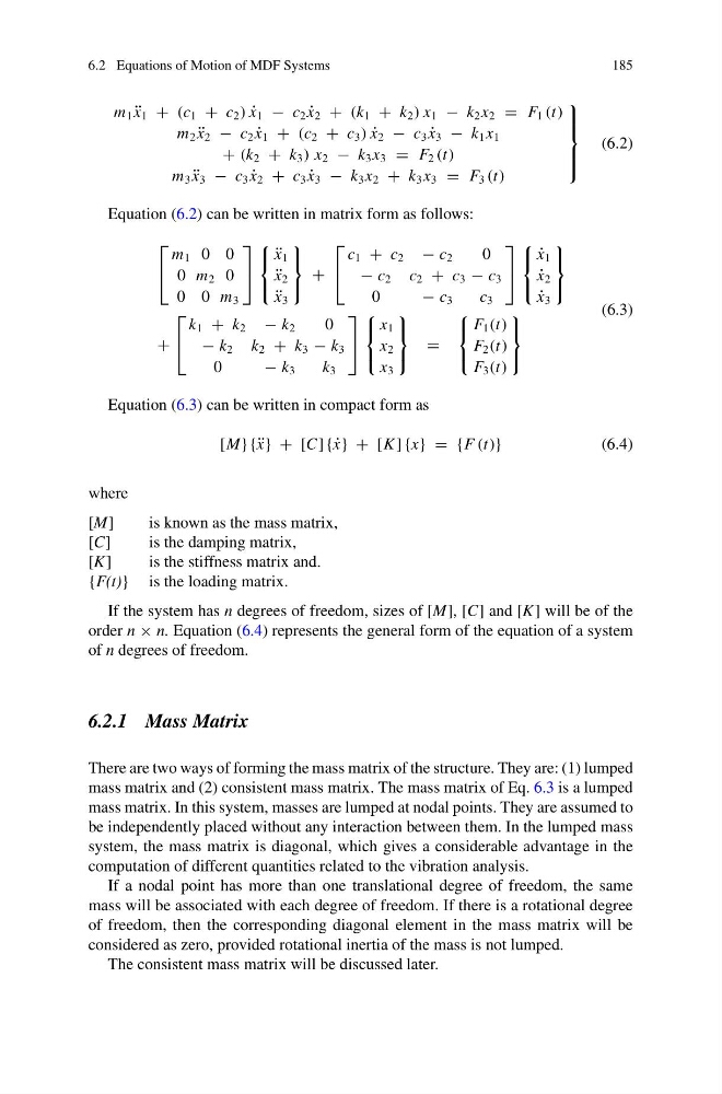
Equation (6.2) can be written in matrix form as follows:
⎡
⎣
m 1 0 0
0 m 2 0
0 0 m 3
⎤
⎦
⎧
⎨
⎩
¨
x 1
¨
x 2
¨
x 3
⎫
⎬
⎭
+
⎡
⎣
c 1 + c 2 − c 2
0
− c 2 c 2 + c 3 − c 3
0
− c 3
c 3
⎤
⎦
⎧
⎨
⎩
˙
x 1
˙
x 2
˙
x 3
⎫
⎬
⎭
+
⎡
⎣
k 1 + k 2 − k 2
0
− k 2 k 2 + k 3 − k 3
0
− k 3
k 3
⎤
⎦
⎧
⎨
⎩
x 1
x 2
x 3
⎫
⎬
⎭
=
⎧
⎨
⎩
F 1 (t)
F 2 (t)
F 3 (t)
⎫
⎬
⎭
(6.3)
Equation (6.3) can be written in compact form as
[M} { ¨
x} + [C] { ˙
x} + [K ] {x} = {F (t)}
(6.4)
where
[M]
is known as the mass matrix,
[C]
is the damping matrix,
[K]
is the stiffness matrix and.
{F(t)} is the loading matrix.
If the system has n degrees of freedom, sizes of [M], [C] and [K] will be of the
order n × n. Equation (6.4) represents the general form of the equation of a system
of n degrees of freedom.
6.2.1 Mass Matrix
There are two ways of forming the mass matrix of the structure. They are: (1) lumped
mass matrix and (2) consistent mass matrix. The mass matrix of Eq. 6.3 is a lumped
mass matrix. In this system, masses are lumped at nodal points. They are assumed to
be independently placed without any interaction between them. In the lumped mass
system, the mass matrix is diagonal, which gives a considerable advantage in the
computation of different quantities related to the vibration analysis.
If a nodal point has more than one translational degree of freedom, the same
mass will be associated with each degree of freedom. If there is a rotational degree
of freedom, then the corresponding diagonal element in the mass matrix will be
considered as zero, provided rotational inertia of the mass is not lumped.
The consistent mass matrix will be discussed later.
185
m 1 ¨
x 1 + (c 1 + c 2 ) ˙
x 1 − c 2 ˙
x 2 + (k 1 + k 2 ) x 1 − k 2 x 2 = F 1 (t)
m 2 ¨
x 2 − c 2 ˙
x 1 + (c 2 + c 3 ) ˙
x 2 − c 3 ˙
x 3 − k 1 x 1
+ (k 2 + k 3 ) x 2 − k 3 x 3 = F 2 (t)
m 3 ¨
x 3 − c 3 ˙
x 2 + c 3 ˙
x 3 − k 3 x 2 + k 3 x 3 = F 3 (t)
⎫
⎪ ⎪ ⎬
⎪ ⎪ ⎭
(6.2)
Equation (6.2) can be written in matrix form as follows:
⎡
⎣
m 1 0 0
0 m 2 0
0 0 m 3
⎤
⎦
⎧
⎨
⎩
¨
x 1
¨
x 2
¨
x 3
⎫
⎬
⎭
+
⎡
⎣
c 1 + c 2 − c 2
0
− c 2 c 2 + c 3 − c 3
0
− c 3
c 3
⎤
⎦
⎧
⎨
⎩
˙
x 1
˙
x 2
˙
x 3
⎫
⎬
⎭
+
⎡
⎣
k 1 + k 2 − k 2
0
− k 2 k 2 + k 3 − k 3
0
− k 3
k 3
⎤
⎦
⎧
⎨
⎩
x 1
x 2
x 3
⎫
⎬
⎭
=
⎧
⎨
⎩
F 1 (t)
F 2 (t)
F 3 (t)
⎫
⎬
⎭
(6.3)
Equation (6.3) can be written in compact form as
[M} { ¨
x} + [C] { ˙
x} + [K ] {x} = {F (t)}
(6.4)
where
[M]
is known as the mass matrix,
[C]
is the damping matrix,
[K]
is the stiffness matrix and.
{F(t)} is the loading matrix.
If the system has n degrees of freedom, sizes of [M], [C] and [K] will be of the
order n × n. Equation (6.4) represents the general form of the equation of a system
of n degrees of freedom.
6.2.1 Mass Matrix
There are two ways of forming the mass matrix of the structure. They are: (1) lumped
mass matrix and (2) consistent mass matrix. The mass matrix of Eq. 6.3 is a lumped
mass matrix. In this system, masses are lumped at nodal points. They are assumed to
be independently placed without any interaction between them. In the lumped mass
system, the mass matrix is diagonal, which gives a considerable advantage in the
computation of different quantities related to the vibration analysis.
If a nodal point has more than one translational degree of freedom, the same
mass will be associated with each degree of freedom. If there is a rotational degree
of freedom, then the corresponding diagonal element in the mass matrix will be
considered as zero, provided rotational inertia of the mass is not lumped.
The consistent mass matrix will be discussed later.